An IB Method for Non-Newtonian-Fluid Flexible-Structure Interactions in Three-Dimensions

Luoding Zhu

1 Indiana University-Purdue University Indianapolis,USA.

Abstract: Problems involving fluid flexible-structure interactions(FFSI)are ubiquitous in engineering and sciences.Peskin’s immersed boundary(IB)method is the first framework for modeling and simulation of such problems.This paper addresses a three-dimensional extension of the IB framework for non-Newtonian fluids which include power-law fluid,Oldroyd-B fluid,and FENE-P fluid.The motion of the non-Newtonian fluids are modelled by the lattice Boltzmann equations(D3Q19 model).The differential constitutive equations of Oldroyd-B and FENE-P fluids are solved by the D3Q7 model.Numerical results indicate that the new method is first-order accurate and conditionally stable.To show the capability of the new method,it is tested on three FFSI toy problems:a power-law fluid past a flexible sheet fixed at its midline,a flexible sheet being flapped periodically at its midline in an Oldroyd-B fluid,and a flexible sheet being rotated at one edge in a FENE-P fluid.

Keywords: Fluid flexible-structure interaction,immersed boundary method,lattice Boltzmann,power-law,Oldroyd-B,FENE-P.

1 Introduction

Phenomena of fluid flexible-structure interactions (FFSI) are ubiquitous in various fields of engineering and sciences.For instances,clothes moving in a washing machine,booms floating in ocean preventing oil pollution,blood flowing in deformable blood vessels,to name just a few.Due to complexity of such problems,mathematical modeling and computer simulation of FFSI problems are challenging.The first methodology for modeling and simulation of FFSI problems is probably the immersed boundary (IB)method introduced by Peskin [Peskin (1972,1973)].Since the birth of the IB method,numerous methods for FFSI problems are developped.These include immersed boundary method[Iaccarino and Verzicco(2003);Mittal and Iaccarino(2005)],Arbitrary Lagrangian Eulerian (ALE) [Hughes,Liu and Zimmermann (1981);Donea,Giuliani and Halleux(1982);Yang,Sun,Wang et al.(2016)],the lattice Boltzmann[Lallemand and Luo(2003)],fictitious domain [Glowinski,Pan and Periaux (1994a,b)],front tracking [Glimm,Grove,Li et al.(1998)],immersed interface[Leveque and Li(1994);LeVeque and Li(1997);Li and Lai(2001)],blob-projection[Cortez(2000)],phase field[Sun,Xu and Zhang(2014);Wick(2016);Zheng and Karniadakis(2016);Mokbel,Abels and Aland(2018)],immersed finite element[Zhang,Gerstenberger,Wang et al.(2004);Liu,Tang et al.(2007)],material points[Sulsky,Chen and Schreyer(1994);Sulsky,Zhou and Schreyer(1995)],immersed continuum[Wang and Liu(2004);Wang(2006)],the level set[Hou,Li,Osher et al.(1997);Xu,Li,Lowengrub et al.(2006);Cottet and Maitre (2006)],the gas-kinetic [Jin and Xu(2008)],and monolithic approach[Hübner,Walhorn and Dinkler(2004);Hron and Turek(2006);Barker and Cai(2010)].

Because of complexity and diversity of FFSI problems and limitations of mathematics and computer technology,the immersed boundary method has had many different variants designed specifically for FFSI problems with various peculiar features.Examples include the original versions[Peskin(1972,1977);Peskin and McQueen(1996)],the compressible fluid version [Wang,Currao,Han et al.(2017)],the fluid-solute version [Lee,Griffith and Peskin (2010)],the rigid body version [Kim and Peskin (2016)],the thick rod version [Lim,Ferent,Wang et al.(2008)],the volume-conservation version [Peskin and Printz(1993);Rosar and Peskin(2001)],the poroelastic version[Strychalski,Copos,Lewis et al.(2015)],the adaptive mesh-refinement [Roma,Peskin and Berger (1999);Griffith,Hornung,McQueen et al.(2007)],the porous media [Stockie (2009)],the formally 2ndorder[Lai and Peskin(2000);Griffith and Peskin(2005)],the multigrid [Zhu and Peskin(2002);Zhu and Chin (2008)],the penalty [Kim and Peskin (2007)],the finite element[Boffiand Gastaldi (2003);Boffi,Gastaldi,Heltai et al.(2008);Griffith and Luo (2012);Hua,Zhu and Lu(2014)],the stochastic [Atzberger,Kramer and Peskin(2007);Atzberger and Kramer(2008)],the lattice-Boltzmann [Feng and Michaelides(2004,2005);Zhu,He,Wang et al.(2011a);Tian,Luo,Zhu et al.(2011);Cheng and Zhang(2010);Wu and Shu(2009);Shu,Liu and Chew (2007);Niu,Shu,Chew et al.(2006);Wu,Shu and Zhang(2010);Cheng,Zhu and Zhang(2014);Liu,Peng,Liang et al.(2012);Zhang,Cheng,Zhu et al.(2016)],the variable viscosity version [Fai,Griffith,Mori et al.(2013,2014)],the vortex-method version [McCracken and Peskin (1980)],the implicit versions [Fauci and Fogelson(1993);Taira and Colonius(2007);Mori and Peskin(2008);Hou and Shi(2008);Newren,Fogelson,Guy et al.(2008);Hao and Zhu(2010,2011)],

Newtonian fluids are assumed for most of the existing versions of the IB method.However,FFSI problems may involve non-Newtonian fluids.For instance,cytoplasm interacting with cytoskeleton in a living cell;blood interacting with red/white cells in a blood vessel;and poroelastic tissue interacting with a cancer cell during metastasis.Many special properties are displayed by non-Newtonian fluids including normal stress differences and shear thinning/thickening.In contrast to Newtonian fluids which may be described by a universal strain-stress equation;there exists no universal constitutive equation for all non-Newtonian fluids.Different non-Newtonian fluids have to be described by different constitutive equations (algebraic or differential) characterizing history effects and strainstress relationships.

Note that the existing non-Newtonian immersed boundary methods [Chrispell,Cortez,Khismatullin et al.(2011);Chrispell,Fauci and Shelley(2013);Tian(2016);Zhu,Yu,Liu et al.(2017)] are for power-law or Oldroyd-B fluids in two-dimensions except [Zhu,Yu,Liu et al.(2017)]which is three-dimensional for power-law fluids.Tian et al.[Ma,Wang,John et al.(2018)] are developping an immersed-boundary lattice-Boltzmann method for viscoelastic fluids including Oldroyd-B and FENE-CR fluids.In their work the motion equations of the solid are solved for by finite difference or finite element methods.In this paper we discuss our recent development of a 3D IB methods for three non-Newtonian fluids:power-law,Oldrod-B[Oldroyd(1950)],and FENE[Peterlin(1961)].These models can describe many non-Newtonian fluids encountered in real-world problems including blood and polymeric fluids.Some preliminary results was reported in a short letter [Zhu(2018)].Details and more tests of the new method,including the integration of the three non-Newtonian models are presented in the current paper.

In our new method,the lattice Boltzmann equations,the D3Q19 model [Qian (1990);SY and GD (1998)],are used to model the fluid flow.The power-law,the Oldroyd-B model,and the FENE-P model are used to model constitutive equations for various non-Newtonian fluids.The formal one(power-law)is incorporated into the lattice Boltzmann D3Q19 model by an algebraic approach;the latter two are numerically solved by the lattice Boltzmann D3Q7 model[Malaspinas,Fiétier and Deville(2010)].The deformable structure is modelled by elastic fibers which can be stretched,compressed,and bent.The fluid-structure-interaction is modelled by the Dirac delta function,as in Peskin’s original immersed boundary method.Note that in our method,the three non-Newtonian models are integrated seamlessly via a model parameter.Selection of a specific model is done by setting a specific numerical value to the parameter.This is a unique feature of our hybrid method thanks to the advantages of using lattice Boltzmann approach for modeling both fluid motions and the corresponding constitutive equations.

To examine the new method and demonstrate its capability,we consider three FFSI toy problems- a power-law fluid flow passes a deformable sheet tethered at the middleline,a flexible rectangular sheet is flapped sinusoidally at its midline in a stationary Oldroyd-B fluid,and a flexible rectangular sheet is rotated at one edge in a stationary FENE-P fluid.The remaining article is as follows.Section 2 gives the complete mathematical formulation of the IB method for non-Newtonian fluids.Section 3 discusses details of the numerical methods for the mathematical formulation.Section 4 addresses the verification and validation of the new method and its implementation.Section 5 reports some main simulation results for each of the three test problems.Section 6 concludes the paper with a summary.

2 Mathematical formulation

The immersed boundary formulation,a nonlinear system of differential-integral equations,describing the motion of a generic flexible structure in a non-Newtonian fluid(power-law,Oldroyd-B or FENE-P)may be written as follows.The equations are listed first and then followed by explanation.

Eqs.(1)and(2)are the classic Navier-Stokes equations for a viscous incompressible fluid where u denotes the fluid velocity,ρdenotes the density,pthe pressure.The symbolfibdenotes the Eulerian force applied by the immersed structure to the fluid,bfdenotes other external forces exerted on the fluid,for example,the gravity.The letter D=(∇u+∇uT)/2 denotes the strain rate tensor,ηthe fluid dynamic viscosity,and Π the viscoelastic stress tensor.Note that the two equations are valid for both Newtonian and non-Newtonian fluids.For Newtonian fluids,ηis constant and Π is zero.For non-Newtonian fluids obeying power-law,ηis given by Eq.(3) whereis the shear rate,Dijis theijthcomponent of strain rate tensor,constantsη0andnare model parameters describing the properties of the non-Newtonian fluid.Note that whenn= 1 the fluid becomes Newtonian.For non-Newtonian fluids such as polymeric fluids,the viscoelastic stress Π may be computed from the conformation tensorC(Eq.(4)),whereκpandµpare the relaxation time and dynamical viscosity of the polymer,respectively.The polymer conformation tensorCis governed by Eq.(4),i.e.,the FENE-P model[Peterlin(1961)].The variablesaandbare given by Eq.(5) whererpis a model parameter related to the maximum length of polymer molecules which is permitted andtr(C)is the trace of the conformation tensorC.Note that variableais a nonlinear function of the conformation tensorCand the FENE-P model is a nonlinear system of hyperbolic partial differential equations.Whena=b= 1,FENE-P model reduces to the popular linear Oldroyd-B model [Oldroyd (1950)].Note that the Navier-Stokes equations are parabolic and elliptic in nature,but the FENE-P model (Eq.(4)) is hyperbolic.They are coupled through fluid velocity u and viscoelastic force Π.

The immersed boundary Eulerian force densityfibin Eqs.(1)and(2)can be computed via Eq.(6),whereαis the Lagrangian coordinate of the immersed structure.The functionδis the classic Dirac delta function.The symbolXis Lagrangian position of the structure.The function F is the corresponding Lagrangian force density,which is computed from the elastic potential energies (Eq.(8)) of the structure.In Eq.(8),the first integral represents the contribution from stretching/compression(Es)and the second one represents the contribution from bending(Eb).The quantitiesKbandKsare bending and stretching coefficients of the elastic constitutive fibers of the deformable structure.Their numerical values are related to the Youngs’modulus and Poisson ratio of the structure[Strychalski,Copos,Lewis et al.(2015)].The velocity of the immersed structureU(α,t)is interpolated from the velocity of surrounding fluid by Eq.(10).Note that this equation by definition dictates that the immersed structure must follow the motion of fluid because of fluid viscosity.That is,the no-slip boundary condition is enforced on the fluid-solid interface.There are three major dimensionless ratios in the FFSI problems involving non-Newtonian fluids:Reynolds numberstructure flexure modulusa nd Weissenberg number for polymeric fluidWi=κp(or exponentnfor power-law fluid).In above definition,ρcis the characteristic fluid mass density,Ucis the characteristic flow speed,Lcis the characteristic length of the immersed structure,κpis the relaxation time of polymer,is the characteristic flow shear rate,νpis the polymer kinematic viscosity,andνfis the fluid kinematic viscosity.Note thatRemeasures the ratio of inertial force and viscous force,measures the ratio of the elastic force and inertial force,Wimeasures the ratio of viscoelastic force and viscous force.The index of power-lawn<1 corresponds to shear-thinning fluid,n >1 corresponds to shear-thickening fluid,andn= 1 corresponds to Newtonian fluid.

3 Numerical methods

As we can see,the immersed boundary formulation for the FFSI problems of non-Newtonian fluids is a nonlinear system of integral and partial differential equations(PDE).The PDEs are of mixed type (hyperbolic,parabolic,and elliptic).Numerical solution of this kind of hybrid system is challenging.Here we choose to use the lattice Boltzmann approach [Wolf-Gladrow (2000);Guo and Shu (2013);Huang,Sukop and Lu (2015);Succi (2018)] for this system.The lattice Boltzmann approach treats the incompressible flows as slightly compressible flows (which are governed by hyperbolic PDEs).This kind of artificial compressibility approach for the flow equations is consistent with the hyperbolic nature of the constitutive equations of the non-Newtonian fluids such as FENEP fluids.The details of the discretizations for the flow equations,constitutive equations,and immersed boundary equations are given as below.

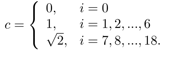
The lattice Boltzmann equations,the D3Q19 model[Qian(1990);SY and GD(1998)],are used to solve numerically the viscous incompressible flow equations (Eqs.(1) and (2))for non-Newtonian fluids.Carefully chosen 19 velocities (with three speeds) are used to discretize the particle velocity spaceξ,ξi(i=0,1,...,18):

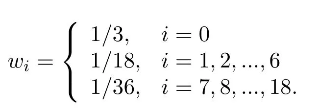
Usegi(x,t)to denote the single-particle velocity distribution function along the direction ofξi(i=0,1,...,18).The lattice Boltzmann equation(LBE)advancinggi(x,t)one-timestep forward along the directionξican be written as

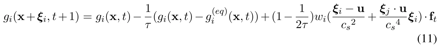
Here ft=fib+∇·Π+fb.The relaxation timeτis related to the fluid kinematic viscosityThe weightwiis given as follows:

The functionis the discretization of the equilibrium distribution function:

The method introduced in Guo et al.[Guo,Zheng and Shi (2002)] is applied to treat the external force term.Note that the lattice Boltzmann equation (Eq.(11)) can be regarded as an explicit second-order accurate discretization in space and time of the flow equations for viscous non-Newtonian fluids by a Lagrangian approach [Wolf-Gladrow (2000)].It is equivalent to a second-order finite difference scheme for the viscous incompressible Navier-Stokes equations[Junk(2001)].

For non-Newtonian fluids modelled by power law,the constitutive equation is incorporated into the lattice Boltzmann flow model (the D3Q19) algebraically by Eq.(3).The shear rate may be calculated as follows:is computed bywhereHeregkis the velocity distribution function alongkthdirection,g(eq)kis the equilibrium distribution function,andξki(k= 0,1,...,18;i= 1,2,3) is theithcomponent of thekthdiscrete direction.See[Zhu,Yu,Liu et al.(2017)]for details.

For non-Newtonian fluids whose constitutive laws obeying the FENE-P model(including the Oldroyd-B model),the lattice Boltzmann D3Q7 model for advection-diffusion equations [Malaspinas,Fiétier and Deville (2010)] is applied for numerical solutions of their constitutive equations.It is coupled with the lattice Boltzmann model for flow equations through the flow velocity u and viscoelastic force Π.Lattice Boltzmann particles in the D3Q7 model are allowed to move along six discrete directionsζi,i=1,2,...,6 at a node,where

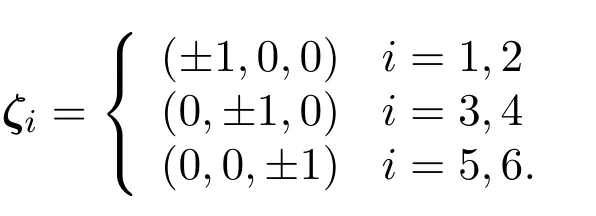
Particles can also stay at the nodeζ0= (0,0,0).For a given component of the configuration tensorCαβ,at a given node x,along a given directionζi,i= 0,1,2,...,6,the single-particle velocity distribution functionqαβiis evolved according to

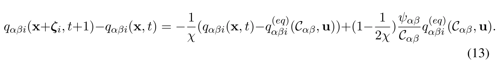
Where the relaxation timeχis related to the diffusivity constantκpThe ratioκp/µpis set to be a very small number e.g.10−6,hereµpis polymer dynamical viscosity.The equilibrium distributionwhereζikis thekth(k= 1,2,3)component of velocityζi(i= 0,1,2,...,6).FunctionTheαβthcomponent of the conformation tensor is computedThe viscoelastic force in Eq.(1)is computed by∇·Π =and the spatial derivative∂xi,i= 1,2,3 is discretized by the central difference scheme.

The macroscopic fluid mass densityρ(x,t)and momentum(hence velocity)ρu(x,t)can be computed fromgi(x,t)at each node by

Let integer m denote time step:gm=g(x,ξ,m),Xm(α) = X(α,m),um= u(x,m),pm=p(x,m),ρm=ρ(x,m).Let the flexible structure be discretized by a set of elastic fibers with Lagrangian coordinateα2.Letα2=k2∆α2,wherek2is an integer.Let a fiber be discretized by a set of points with Lagrangian coordinateα1.Letα1=k1∆α1,wherek1is an integer.

Then the elastic potential energy is discretized by:

where the first term corresponds to the stretching/compression energy and the second term corresponds to the bending energy.The Lagrangian force density at node with indexl,(F)l,l=1,2,...,Nf,is given by

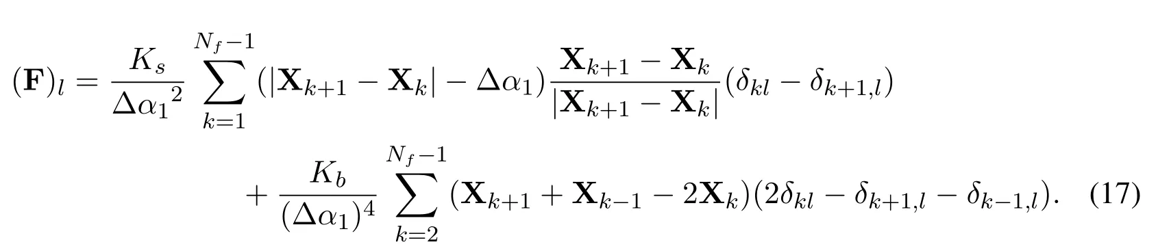
Hereδklis the Kroneckerδ:δkl= 1 ifk=landδkl= 0 if.The integral equations in the immersed boundary formulation are computed by the trapezoidal rule:

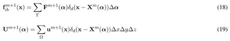
Here Γ denotes the immersed structure,Ω denotes the fluid domain.And ∆x,∆y,and ∆zdenote the meshwidth inx,y,andzdirections.The Diracδfunction is discretized byδd:

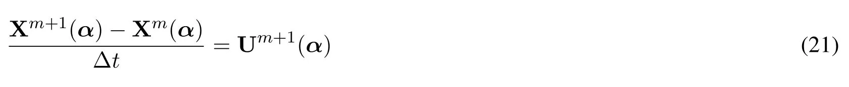
Hereφ(r) = 0.25(1+cos(0.5πr)) for|r| ≤2 and is 0 otherwise.For other choices ofφ(r)see Peskin et al.[Peskin and McQueen(1996)].The motion equation of the structure is discretized by

For clarity the algorithm of the IB formulation for non-Newtonian fluids is summarized as follows.Suppose all variables are known at time step t (an integer),the procedure for updating all of the variables for next time step t+1 is as follows.

0)Initialization of all variables;

1)Advance the LBE(Eq.(11))for flow(D3Q19 model)from t to t+1 using fiband Π from time step t;compute the new fluid velocity u,velocity gradient∇u,and mass densityρ;

2)Advance the LBE(Eq.(13))for the constitutive equations(the D3Q7 model)from t to t+1 using u andCfrom time step t;compute the viscoelastic force∇·Π from the newly updated conformation tensorC,

3)Compute the structure velocity U from the fluid velocity u by Eq.(19);

4)Update the structure position by its velocity via Eq.(21);

5)Compute the immersed boundary force exerted by the structure to the fluid using its new configuration via Eq.(17);

6)Convert the Lagrangian force to Eulerian force by Eq.(18);

7)Compute the new equilibrium distribution functions of theandg(eq)using the newly obtained fluid velocity u,conformation tensorC,and mass densityρ;

8)Go to 1).

Note that the algorithm for non-Newtonian fluids can be easily combined with algorithm for Newtonian fluids using the D3Q19 model.Therefore,the new method may be implemented in one computer program with a single model parametermp(an integer)to switch between Newtonian and non-Newtonian fluids.The optionmp= 0 selects Newtonian fluid.The code will bypass the D3Q7 model and set Π = 0,n= 1.The optionmp= 1 selects the power-law fluid.The code will bypass the D3Q7 model and set Π=0.The optionmp=2 selects the Oldroyd-B fluid.The code will execute the D3Q7 model witha=b= 1 and setn= 1.The optionmp= 3 selects the FENE-P fluid.The code will execute the D3Q7 model and setn= 1.Thus the Newtonian,power-law,Oldroyd-B,and FENE-P fluids are seamlessly integrated together in the new IB method via the lattice Boltzmann approach and they can be implemented in a single computer code.

4 Verification and validation

The numerical methods involved and their implementations used in the work have been verified and validated in different settings.The lattice Boltzmann method (D3Q19) and its implementation have been verified and validated in Zhu et al.[Zhu,Tretheway,Petzold et al.(2005)].The lattice-Boltzmann immersed-boundary method (LB-IB) with its implementation for Newtonian fluid flows have been verified and validated in Zhu et al.[Zhu,He,Wang et al.(2011b)].The LB-IB for power-law fluid is verified and validated in Zhu et al.[Zhu,Yu,Liu et al.(2017)].The preliminary verification and validation of the LB-IB method for Oldroyd-B/FENE-P have been reported in a short letter [Zhu (2018)].In this paper,the newly developped LB-IB method for polymeric flows are further tested on two new FFSI toy problems:a flexible sheet being flapped periodically at the middle and being rotated constantly at one edge in stationary Oldroy-B and FENE-P fluids in three dimensions.Many simulations with various dimensionless parameters indicate that the method is conditionally stable.Mesh refinement studies indicate the method is first-order accurate,which is consistent with the IB framework in general.

5 Test problems

In this section we consider three FFSI model problems.I)a power-law fluid flows around a flexible rectangular sheet fixed at the midline in a three-dimensional rectangular domain;II)a flexible rectangular sheet is flapped sideways(left and right)at the midline sinusoidally in a 3D rectangular box full of an Oldroyd-B;III) a flexible rectangular sheet is rotated constantly at one edge with a constant speed in a 3D rectangular box full of a FENE-P fluid.

In case I,the structure is initially stationary.The flow passes around it and causes it to bend and get aligned with the flow.No-slip boundary condition is applied on the top,bottom,front,and rear rigid walls.Constant velocity is specified at the inlet and outlet boundaries(inx-axis).In cases II and III,the fluid is initially stationary and the structure is forced to move.The active motions of the structures drive the fluid flow.Periodic boundary condition is applied along all directions of the computational domain.In all cases,thex−axis points from left to right;they−axis points from front to rear;thez−axis points from bottom to top.The sheets are composed of two groups of elastic fibers which can be compressed,stretched,and bent.The two groups of fibers are cross-linked and are orthogonal to each other initially.This type of FFSI problem possesses three significant dimensionless parameters:flow Reynolds numberRe,structure bending modulusand fluid Weissenberg numberWi(or exponentnfor power-law fluid).Numerous simulations on the three model problems using various combinations of these parameters are performed to test the capability of the new method.Some representative simulation results are reported below for each case.

Case I)An elastic sheet with aspect ratio 1:2(width versus length)is placed initially on they−zplane(i.e.,vertical)in the middle of the box(inx,y,andzdirections).Its midline is fixed in a power-law fluid flow and the sheet is free to move otherwise.This problem was intensively studied by Zhu et al.[Zhu,Yu,Liu et al.(2017)].More simulations are performed and some typical results from different combination of values ofRe,nare shown here.The left panel in Fig.1 shows the position and shape of the sheet at several equally distributed time instants from a simulation withRe= 80,b= 0.0001,n= 0.5.The left most is the initial position(vertical and flat).The right most is the final position(curved).Starting from the initial configuration,the sheet moves and deforms with the flow,and finally sets down to a quasi-steady state.Note that the position/shape of the sheet partially overlap for some instants.The right panel in Fig.1 shows streamlines of the flow field from a simulation withRe= 120,b= 0.05,n= 0.6.The gray surface is the position and shape of the sheet.The streamlines start from the lower half plane of the inlet(using tens of uniformly spaced seeds).Notice the twisted curves behind the sheet.These streamlines come from the lower half plane at inlet and move to the upper half plane after past the sheet.This reveals the complicated flow patterns right behind the sheet.

Figure 1:Position and shape of the sheet at several instants(left)and streamlines(right)

Case II) A deformable sheet of the same aspect ratio is initially placed the same way as in case I.Its midline is now forced to flap sinusoidally (on thex−yplane alongx-direction) in an Oldroyd-B fluid.Thex-coordinate of the leading edge is given byHerex(t) is thex-coordinate of the sheet middle-line,A denotes prescribed amplitude of flapping,P denotes flapping period,and t denotes time.Some typical results from different combination of values ofRe,,Wiare given below.In Fig.2 the left panel plots the shape of the sheet at several equally separated instants from a simulation withRe= 40,b= 0.005,Wi= 0.1.The left most is the initial position(vertical and flat).The rest is the shape(not physical position)of the sheet at several time instants within a period.Note that the sheet physical position (x-coordinate) is shifted horizontally by a constant for the purpose of displaying the shapes at multiple instants on the same panel.Starting from the initial position,the sheet moves and deforms with the flapping midline.Spontaneous motion of the sheet alongyandzdirections are not seen.The right panel in Fig.2 shows streamlines of the flow field from a simulation withRe= 60,b= 0.004,Wi= 0.1.The gray surface(partially buried in the curves)at the center is the position and shape of the sheet.All streamlines start from a vertical plane(parallel to the initial position of the sheet) near the left boundary of the computational domain (using 25 uniformly spaced seeds).Notice the colors of the curves denote the velocity magnitude.The twisted curves around the sheet indicates the complexity of flow patterns in the vicinity of the structure.

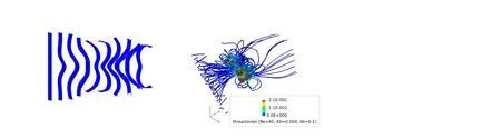
Figure 2:Shape of the sheet at several instants(left)and streamlines(right)

Case III)An elastic sheet with aspect ratio of 1:4(width versus length)is initially put on a horizontal plane of thexandyaxes in the middle of the box in all three directions (x,y,andz).Its right edge is rotated constantly and periodically with a periodP(on they−zplane anticlockwise) in a still FENE-P fluid.Again,the structure is not restricted elsewhere and is allowed to move freely in other directions.Some typical results from different combination of values ofRe,,Wiare displayed here.In Fig.3 the left panel shows the shape/position of the sheet at a few equally distributed instants from a simulation withRe=10,b=0.005,Wi=1.0.The top most is the initial position(horizontal and flat).The remaining is the shape(not physical position)of the sheet at several time instants within a period.Note that the sheet vertical position is shifted down by a constant for the same purpose as in case II.We see that as the right edge is being rotated,the rest of the sheet follows the rotation motion.Due to flexibility (instead of being rigid),the leading edge (initially straight) deforms into a curve and the entire sheet deforms into a helical structure.As time goes by,more helical structures appear and they appear to move downstream(from righ to left)in an animation.Interestingly the entire sheet moves forward towards right boundary slowly.The right panel in Fig.3 shows streamlines of the flow field from a simulation withRe= 10,b= 0.005,Wi= 1.0.The gray surface (partially blocked by the curves)is the position and shape of the twisted sheet.All streamlines start from a horizontal plane parallel and close to the initial position of the sheet(20 uniformly spaced seeds).The colors of the curves denote the velocity magnitude.The tightly wound curves around the sheet indicate a rotating flow near the sheet.

Figure 3:Shape of the sheet at several instants(left)and streamlines(right)

6 Summary

The existing immersed boundary (IB) framework has been extended in three dimensions to FFSI problems involving non-Newtonian fluids.The fluids may be power-law,Oldroyd-B,or FENE-P.The viscous incompressible Navier-Stokes equations for the flow and the constitutive equations for the fluid (Oldroyd-B and FENE-P) are simultaneously solved with the lattice Boltzmann approaches by the D3Q19 and the D3Q7 models,respectively.The power-law is incorporated algebraically into the lattice Boltzmann flow model.The new method is tested on three FFSI toy problems:deformable sheets interacting with power-law,Oldroyd-B,and FENE-P fluids in three dimensions.Our results show that the new IB method is first-order accurate and conditionally stable.

Acknowledgment:The work is supported by the US National Science Foundation(NSF)through the research grant DMS-1522554.We thank the unknown Reviewers for their helpful suggestions and comments which have helped us.