OpenIFEM:A High Performance Modular Open-Source Software of the Immersed Finite Element Method for Fluid-Structure Interactions

Jie Cheng,Feimi Yu and Lucy T.Zhang, *

1 Department of Mechanical Aerospace and Nuclear Engineering,Rensselaer Polytechnic Institute,Troy,NY,12180,USA,

Abstract: We present a high performance modularly-built open-source software -OpenIFEM.OpenIFEM is a C++implementation of the modified immersed finite element method (mIFEM) to solve fluid-structure interaction (FSI) problems.This software is modularly built to perform multiple tasks including fluid dynamics (incompressible and slightly compressible fluid models),linear and nonlinear solid mechanics,and fully coupled fluid-structure interactions.Most of open-source software packages are restricted to certain discretization methods;some are under-tested,under-documented,and lack modularity as well as extensibility.OpenIFEM is designed and built to include a set of generic classes for users to adapt so that any fluid and solid solvers can be coupled through the FSI algorithm.In addition,the package utilizes well-developed and tested libraries.It also comes with standard test cases that serve as software and algorithm validation.The software can be built on cross-platform,i.e.,Linux,Windows,and Mac OS,using CMake.Efficient parallelization is also implemented for high-performance computing for large-sized problems.OpenIFEM is documented using Doxygen and publicly available to download on GitHub.It is expected to benefit the future development of FSI algorithms and be applied to a variety of FSI applications.

Keywords: Immersed finite element method,open-source,parallelization,fluid-structure interaction,adaptive mesh refinement.

1 Introduction

Fluid-structure interactions are difficult to model as they involve complicated motions and deformations of the fluid-structure interface.Tremendous research efforts have been devoted to developing numerical algorithms for FSI problems since 1970s.One of the early attempts is the Arbitrary Lagrange Eulerian(ALE)method[Hughes,Liu and Zimmermann(1981);Liu and Ma (1982);Liu,Chang,Chen et al.(1988);Hu,Patankar and Zhu(2001)].ALE method requires conforming meshes between fluid and structure,which can handle complicated fluid-solid interface at the cost of expensive mesh-updating and re-meshing.In practice,the difficulty of re-meshing grows with the large displacement and deformation of the fluid-structure interface.To avoid this process,a series of non-conforming techniques have emerged to model FSI problems.One of which is the immersed method which postulates the co-existence of the fluid and the solid domains so that non-conforming meshes or discretizations can be used for the fluid and the structure.Immersed boundary(IB)method is initially developed by[Peskin(1977,2002)],in which solid membrane is modeled as elastic fibers,and described as a set of equivalent body forces in the Navier-Stokes equations.Based on the IB method,immersed interface method is developed by Peskin[Leveque and Li(1994)],which improves the accuracy of the original formulation to capture the pressure jump of the interface.Another derivative of the IB method is the extended immersed boundary method[Wang and Liu(2004)]which replaces the simplistic elastic fiber model with the standard finite element method.Immersed finite element method(IFEM)[Zhang,Gerstenberger,Wang et al.(2004);Zhang and Gay(2007);Wang,Wang and Zhang (2012)],on the other hand,completely changes the formulation so that the immersed domain becomes“volume-based”rather than discrete“point-based”.It models the entire solid volume using finite elements,where the solid occupies a volume and the solid constitutive law is represented.

In all the immersed methods mentioned above,including the immersed finite element method,the solid displacement is imposed from the fluid velocity,rather than being solved from its own governing equations.The modified immersed finite element method(mIFEM) changes the formulation so that the imposition of the velocity is reversed:the solid dynamics is solved using its own governing equation and its velocity is imposed onto its overlapping fluid domain [Wang and Zhang (2013)].Comparing to the original IFEM,which may lead to severe solid mesh distortion resulting in the overestimation of the solid deformation especially for high Reynolds number flows.The mIFEM preserves the solid dynamics by faithfully solving its governing equations,therefore it produces more accurate and realistic coupled solutions.Furthermore,mIFEM does not impose fluid velocity onto the solid,thus removes the incompressibility constraint on the solid when the background fluid is incompressible.An important advantage of the mIFEM is that it is minimally-intrusive to the fluid and solid solvers,which allows modularity in the solvers.The interactions between the solid and the fluid are reflected as tractions on the solid boundary,body force and no-slip boundary conditions in the artificial fluid region.As a result,the information exchange between the fluid and the solid is rather straightforward because the fluid/solid solvers are interfaced to apply those Neumann and Dirichlet boundary conditions.

As the immersed algorithms become further utilized in FSI applications,a number of open-source software packages implementing these algorithms became available.Currently the most developed ones are based on IB method.For example,IB method with Adaptive Mesh Refinement(AMR),namely IBAMR[Griffith(2014)],has been under rapid development for more than 4 years.It uses mainly C++ language.IBAMR has become relatively complete in the sense that it contains many variants of the immersed boundary method,which are specialized to solve bio-membrane types of problems.It has been mainly applied to cardiac blood flows [Battista,Lane and Miller (2017)] as well as swimming and flying animals[Bale,Hao,Bhalla et al.(2014)].Another software package is PetIBM [Chuang,Mesnard,Krishnan et al.(2018)].Different from IBAMR,PetIBM is rather specialized for the Immersed Boundary Projection Method [Wang,Giraldo and Perot(2002)],with applications for only incompressible fluid.cuIBM[Layton,Krishnan and Barba(2011)]is a new immersed boundary method code based on GPU parallelization.cuIBM is currently under development,at the time of writing it is only capable of solving 2D incompressible Navier-Stokes equations.This software is focused on GPU acceleration on a single CUDA-capable device,and shows good speedup for small and medium size problems.Due to the shorter history,currently there is few open-source packages for immersed finite element method.One of them is ans-ifem [Heltai,Roy and Costanzo(2012)].Ans-ifem is a C++implementation of Heltai et al.[Heltai and Costanzo(2012)],which is more of a demonstration rather than a usable software,and is no longer maintained.It comes with several examples that help users understand the algorithm.However,the numerical procedures to solve the fluid and solid governing equations are monolithic in some way,and the entire code is in one piece,which makes it very challenging to modify any part of the code to suit an application.

OpenIFEM will address the following issues that exist in the available FSI software packages:

•Modularity and extensibility:one of the most common problems of the existing projects is the lack of modularity and extensibility,which hinders the customization of the code.Very often,a user wants to plug his/her own numerical model into the software for a certain engineering application.To address this,the components of OpenIFEM are divided into a variety of independent classes that can be replaced by the user,with a set of Application Program Interfaces(APIs)defined from high level to low level to ensure the algorithm still works after customization.At a higher level,it is easy for a user to add a new fluid or solid solver into OpenIFEM without having to change the FSI algorithm.The FSI solver interacts with the fluid and the solid solvers through a small number of APIs such as element-wise body force and traction boundary conditions.The user only needs to ensure the new solver supports these APIs.At a lower level,effort is made in OpenIFEM to account for possible extensions to solid constitutive law,time/space-dependent boundary conditions,etc.Generic classes that handle common routines are written so users can easily derive a new class from them and override these routines.

•Restrictions on discretization techniques:existing projects have restrictions on the numerical methods to solve fluid/solid governing equations.For instance,PetIBM is restricted to Perot’s fractional step method [Perot (1993)] to solve the Navier-Stokes equations;cuIBM also only works with projection method.On the contrary,OpenIFEM does not make assumptions on how the fluid and solid governing equations are solved,as long as they allow standard boundary conditions such as body force to be set.

•Efficiency:OpenIFEM is fully parallelized using MPI.Not all algorithms can be parallelized to the same degree,due to the fact that some algorithms require intense communications among ranks.mIFEM can be sufficiently parallelized because only limited communications are required among processes.For example,the core of mIFEM,i.e.,the evaluation and interpolation of FSI stress,fluid traction,solid velocity etc.,are performed locally on each process,without using information that are only available to other processes.

•Reproducibility:existing FSI modeling projects often do not pay enough attention to the reproducibility.OpenIFEM has a test suite to ensure the computational results are reproducible.So far,it includes 29 test cases which cover various components of the code.These cases are still growing with the increase in participation from developers.All test cases are accompanied with input parameters and descriptions,and can be run with a single command by using CMake’s module ctest,which prevents regressions during developments.

•Documentation:as pointed out in Mesnard et al.[Mesnard and Barba (2017)],open source research software is often poorly documented and unsupported,and on occasion,can be an unreadable mess.OpenIFEM,on the other hand,is well-documented in a consistent style.In particular,the mathematical formulas are explained and viewed in html or pdf format.In addition,the coding style in OpenIFEM follows consistent conventions to improve readability,such as naming of variables,and fixed indentations of lines.

This project aims to provide a flexible,high performance open-source software for IFEM simulations,using the modular mIFEM formulation.To the authors’ knowledge,it is the first time such a comprehensive software is introduced.The rest of paper is organized as follows:in Section 2 we briefly review the mIFEM algorithm.Then in Section 3 we introduce the design of OpenIFEM in detail,where the software work flow,main features,data structures and external tools,as well as the issues related to software license and contributions are explained.Numerical examples for solid solver,fluid solver,and FSI solver are presented in Section 4.Finally,conclusions are drawn in Section 5.

2 A Brief Review of the Modified Immersed Finite Element Method(mIFEM)

The premise of the immersed approaches is that it couples an Eulerian background fluid that is everywhere in the domain with a Lagrangian solid domain that“floats"on top of the fluid.Similar to the original IFEM algorithms,in an FSI computational domain there exists an artifciial fluid domainthat overlaps with the solid domain Ωs.Combined with the real fluid domain Ωf,the entire fluid domain is governed by Navier-Stokes equations and the impact of the solid is reflected in the FSI force.Different from other fluid-driven immersed method,such as the IB or the original IFEM,the mIFEM algorithm has the advantage of capturing soliddynamics,handling large density disparities,and avoiding severe solid mesh distortion in high Reynolds number flows.For this reason,OpenIFEM adopts mIFEM algorithm as the component solvers can be modularly built.The workflow o f mIFEM algorithm is shown in Fig.1.A variety of options for fluid solvers are available including incompressible and slightly compressible fluids,fully implicit and implicit-explicit time schemes etc.Similarly,solid solvers can include different material models and flexible time discretization schemes.For detailed derivation please refer to Zhang et al.[Zhang,Gerstenberger,Wang et al.(2004);Zhang and Gay (2007);Wang,Wang and Zhang (2012);Wang and Zhang (2013)].The FSI process does not intrude the fluid and solid governing equations themselves,except for when applying appropriate and consistent Dirichlet and Neumann boundary conditions.It does not have particular requirements on discretization methods,e.g.,finite volumevs.finite elements.Doing so allows fluid and solid solvers to be treated as black boxes,where the algorithm can be implemented in a modularized way:a solid solver that solves the solid dynamic equations,a fluid solver that solves the fluid dynamic equations,and an FSI solver works as a median to communicate and pass information between solvers.

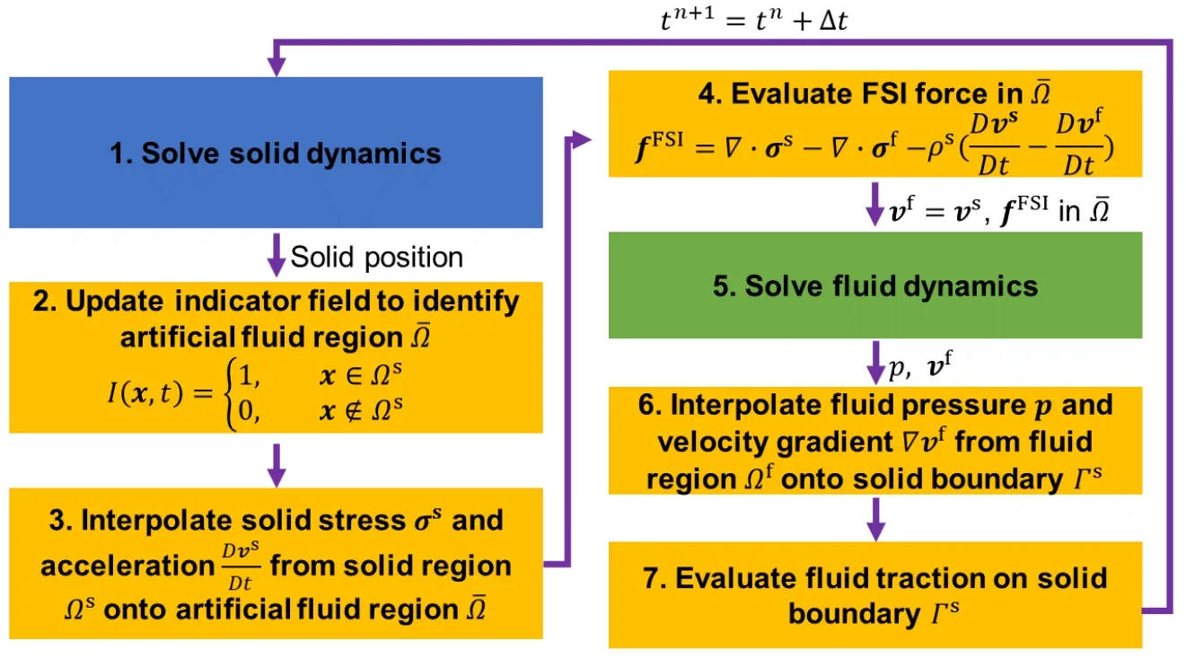
Figure 1:Workflow of the mIFEM algorithm:steps 1 and 5 are independent solid and fluid dynamic solvers,steps 2,3,4,6 and 7 are done by the FSI solver

3 Software design

OpenIFEM is written in C++ with modern design where the components are split into different files and classes to ensure modularity and sustainability,with a clear hierarchical inheritance.In this section,we introduce the structure of OpenIFEM as well as some of its major features.

3.1 Dependencies and tools

OpenIFEM currently includes several finite element solvers:nonlinear solid dynamics,incompressible and compressible fluid dynamics solvers.Both serial and parallel computations using distributed memory are supported.It also includes several additional features such as Adaptive Mesh Refinement(AMR)and user-defined time/space-dependent boundary conditions.We heavily use well-recognized and well-maintained third-party libraries to implement OpenIFEM.The functionalities of these libraries and the justifications of usage are explained below.An illustration of the OpenIFEM dependencies is demonstrated in Fig.2:

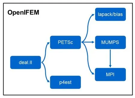
Figure 2:Illustration of software dependencies

deal.II:deal.II [Bangerth,Hartmann and Kanschat (2007)] is a C++ program library that facilitates developers to write programs for solving partial differential equations numerically.It adopts the state-of-the-art programming techniques to provide a large number of data structures and standard routines that are required in finite element methods,such as classes to handle interpolation and integration,routines to reorder the degrees of freedom for efficient matrix solving.Specifically,we use deal.II for its basic data structures in finite element method such as mesh representation,shape functions,Gauss quadrature,etc.OpenIFEM is built upon deal.II to avoid unnecessary tedious work while keeping the core code short and clean.

PETSc:PETSc is a highly optimized linear algebra package created for C/Fortran programs which further depends on other packages such as lapack/blas and MUMPS[Balay,Gropp,McInnes et al.(1997);Balay,Abhyankar,Adams et al.(2017)].PETSc also offers a set of user-friendly APIs to do parallel tasks so that users do not have to concern the details of partition,communication,and synchronization.OpenIFEM relies on PETSc to carry out distributed-memory parallel computations.We further utilize the fact that deal.II has created modern C++wrappers for PETSc data structures that are consistent with the ones of deal.II.By using uniform and consistent data structures,the parallel code looks surprisingly similar to the serial code with minimum intrusion.

p4est:Another important feature in OpenIFEM is the adaptive mesh refinement for enhanced solution accuracy during interfacial solution exchanges.In the design of the IFEM,only the locations of interest,i.e.,in the overlapping region needs to be refined,rather than globally,thus allowing us to investigate interesting details of the computational field without high computational cost.The mesh structure in OpenIFEM is handled by p4est.p4est is a tree-based method [Burstedde,Wilcox and Ghattas (2011)],which makes use of recursive encoding schemes while allowing non-overlapping refinement.Therefore,it combines efficiency and simplicity.We use p4est to deal with mesh refinement and coarsening in both serial and parallel implementations.

3.2 Modularity

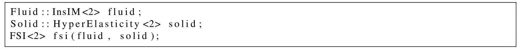
OpenIFEM is designed to solve not only fluid-structure interaction problems but also independent solid mechanics and fluid mechanics problems.The mIFEM algorithm has a natural advantage that it does not pose restrictions on how the fluid governing equations and solid equations should be solved.An FSI simulation runs as long as proper boundary conditions are applied to the fluid solver and solid solver.In the current version,multiple fluid solvers and solid solvers are implemented in OpenIFEM for different applications and all of them can be used in FSI simulation.A typical scenario of Object-Oriented Programming (OOP) is to derive all the fluid solvers from a base class named FluidSolver which handles the common members and methods.Similarly,the solid solvers are derived from a base class named SolidSolver.In an FSI application,a FSI object is constructed,which takes a generic FluidSolver and a generic SolidSolver as members.Any individual fluid or solid solver can be used.This design guarantees the modularity of software components.For instance,the following code snippet demonstrates the combination of a hyperelastic solid solver(Hyperelasticity)and an implicit incompressible Navier-Stokes solver(InsIM):

3.3 Data structures

Various PDEs are solved with finite elements in OpenIFEM,which share a large number of data structures.Among the common data structures,the following are especially important:Triangulation,DoFHandler,FiniteElement,CellProperties and Interpolator,where the first three classes are provided in deal.II and the rest are defined in OpenIFEM.

Triangulation is used to describe a mesh as a hierarchy of levels of elements which may have different refinement levels.It also comes with readers for commonly used mesh generators such as Gmsh and commercial software ABAQUS.

The values of degrees of freedom are stored in a vector.However,in OpenIFEM and other deal.II-based applications,we do not access individual degrees of freedom directly using vector indices.Instead,they are accessed through an intermediate class DoFHandler,which has member functions to query the indices of degrees of freedom residing on vertices,lines,faces,etc.This intermediate layer hides the degrees of freedom indices from the users,so that the users do not have to know the ordering of the degrees of freedom,and DoFHandler can reorder them when necessary.

FiniteElement is the base class for finite element discretization which consists of a number of groups of variables and functions including descriptions of the shape functions and their derivatives;the locations of the supporting points;and the interfaces to evaluate function values and derivatives at an arbitrary point in an element.

CellProperty is a class defined in OpenIFEM to store the cell/quadrature point-specific information.Every element is associated to CellProperty which contains the material properties and can be easily accessed through a pointer.The element-specific properties can be used in the assembly process,thus nonuniform material properties can be easily assigned.In addition,this data structure is used in the FSI process for the FSI force to be expressed as a body force at the integration points.It is set by a FSI object and used as boundary conditions of a FluidSolver object.

Interpolator is a class that performs FSI implementation tasks.During the implementation exchanges,the FSI force is interpolated from the solid nodes onto the fluid quadrature points;the solid nodal velocities are interpolated onto the artificial fluid nodes;the fluid stress is computed at the solid boundary quadrature points to obtain the traction as boundary conditions,which also requires the interpolation of fluid velocity and pressure.Given a DoFHandler and a source vector associated with it,an Interpolator interpolates the source vector to an arbitrary target point:it iterates through the elements and finds the one that contains the target point,then interpolates the source vector to that point using shape functions.At each time step,same interpolation is performed using different source vectors,but Interpolator remembers the element that contains the point and reuses it.

3.4 Input files

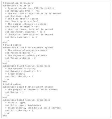
OpenIFEM is currently a terminal-based application that uses text file to specify input parameters.It queries more than 40 input parameters.As the code is further developed,this number is expected to increase.Therefore,a uniform and organized approach to declare and parse input parameters are very essential.

The input parameters are divided into 3 sections:general simulation parameters,fluid-specific parameters,and solid-specific parameters.A ParameterHandler class is used to handle the input parameters.Once an input parameter is declared in this class,it automatically reads the corresponding variable from the input file.Meanwhile,it prints hints on the screen for the user,and checks the validity of the user-provided values.The following text snippet is extracted from a sample input file of OpenIFEM as an example:

3.5 Parallelization

The parallelization of the solvers can be divided into four parts,namely partitioning,assembly,solving and solution output.In OpenIFEM,two kinds of parallelization strategies,distributed mesh and shared mesh,are used for optimal efficiency.Depending on the parallelization strategy deployed,each solver may have slight difference in parallel implementation.We will first go through the process of an individual parallel solver(which can be either fluid or solid solver),then demonstrate the parallelization strategy of the FSI coupling.

PartitioningPartitioning starts at the very beginning of the program.It divides the elements and nodes into partitions,associated to the MPI ranks.An optimal partitioning should have every MPI rank own a continuous chunk of elements,with approxiamtely the same number of degrees of freedom.In all the following procedures,such as assembly,solving linear system,output,each MPI rank is only responsible for its own partition.This is true for both distributed mesh and shared mesh strategies.However,there is a nuance between these two strategies in terms of memory allocation:

•With fully distributed mesh partition,each MPI rank only stores part of the mesh,and part of the vectors,matrices,etc.None of the MPI ranks has full knowledge of the entire mesh.Instead,an MPI rank“owns”some elements,nodes,degrees of freedom etc.that it can read and modify.However,in finite element method,an MPI rank has to communicate with neighboring ranks.The information exchange happens in a“ghost”layer,which covers the direct neighbors of the elements owned by a specific MPI rank.An MPI rank cannot write to,but can read its ghost layer.The values in the ghost elements are set by the MPI ranks that actually“own”them.Distributed mesh partition saves a lot of memory by only storing a portion of the mesh,vectors,matrices etc.While this strategy is scalable,it causes difficulty in the FSI process if both fluid and solid solvers adopt it,which will be explained later in this section.

•Shared mesh partition uses a more straightforward way.Although each rank only writes to its own partition,it has a copy of the entire mesh,so it “knows” the information of the entire domain.It can be thought of as the distributed mesh with a large ghost layer that covers all the elements and nodes that are not locally owned.Comparing to the distributed mesh,it uses more memory on each rank.But if the mesh is not too big to be the bottleneck,it should not cause any problem.The distinction between distributed mesh and shared mesh is shown in Fig.3.

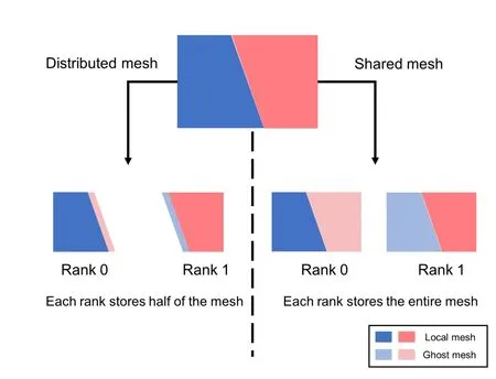
Figure 3:Illustration of distributed mesh and shared mesh

Assembly:In the element-wise assembly process,every rank assembles the local matrices and right hand side vectors for the elements in its partition.Since the partition is continuous,the information required to complete the assembly is local to each rank except for the elements that are on the boundaries of partitions.For those elements,data in other ranks can be accessed through the ghost layer,where only point-to-point communication is involved.The overall communication is insignificant,therefore the workload per rank decreases almost linearly with the number of MPI ranks.As a result,assembly process becomes the most scalable part of the entire program.

Solving:The solving part is done by iterative linear solvers provided inPETSc[Balay,Abhyankar,Adams et al.(2017)].To enable the tailored preconditioners that we use in the fluid solvers,the intermediate matrices should also be assigned and partitioned during the partitioning step.In the iterative linear solvers implemented in PETSc,two types of computations are performed:matrix-vector multiplication and vector norm computation.Since each rank only stores its own part of the matrix and vector,communication is required for both types of computation.While matrix-vector multiplication only involves point-to-point communication,a collective operation is necessary for vector norm computation,which requires heavy communication in the solving part.

Efficiency tests:Two sets of test cases,strong scaling test and weak scaling test,are presented here to evaluate the parallel performance of fluid solver.The test cases are run on DRP cluster located in the Center of Computational Innovation (CCI) at Rensselaer Polytechnic Institute,which consists of 64 nodes with 2 Intel Xeon E5-2650 processors and 128 GB of system memory on each node and connected via 56 GB FDR Infiniband.In the strong scaling test,the total degrees of freedom is set to be around 1.3×106.In the weak scaling test,the degrees of freedom on each rank are fixed to be around 5000,and the problem size grows with MPI ranks.The cases are tested on 1 to 256 MPI ranks(up to 16 nodes).The results of performance tests are shown in Fig.4.In the strong scaling test,the speedup is significant from 1 to 16 cores as only intra-node communication is involved at this stage.In transition from 16 cores to 32 cores,there is a slow-down in the solving time because inter-nodal communication comes into play.For problems larger than 32 cores,the speedup is almost linear with the number of cores.In the weak scaling test,we find that the time for assembly does not change much as the problem size increases.This indicates that assembly has a good scalability as expected.The time for solving increases linearly with the problem size,because iterative solvers have the complexity of orderO(n2),wherenis the number of rows/columns which corresponds to the number of degrees of freedom.Therefore,the linear increase in solving time is also satisfactory.

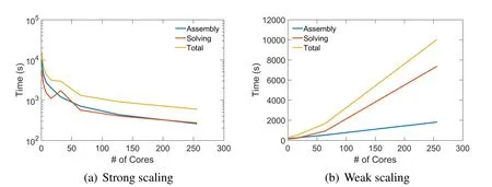
Figure 4:Performance test results

OutputDepending on whether a solver uses distributed mesh or shared mesh,the parallel output process can be different.In a distributed mesh solver,each rank outputs its own data into a .vtu file,which contains only the information on that particular rank.Then a .pvd file is written by rank 0 to indicate all .vtu files to be read.Post-processing software ParaView[Ahrens,Geveci and Law(2005)]then puts together the individual files to accomplish a complete visualization.On the contrary,in a shared mesh solver,rank 0 collects all the results from other ranks.

FSI couplingThe difficulty of FSI parallelization lies in the fact that the iteration of fluid elements and solid elements are nested during the search of the interpolation process.In order to compute the FSI force,for every fluid element,we need to determine whether any of its quadrature points is contained in a solid element (as shown in Algorithm 3.1);similarly,for every quadrature point on a solid boundary,we need to search which fluid element it is immersed in,so that the traction applied to the solid boundaries can be computed(as shown in Algorithm 3.2).Because of the nested loops during the search over both fluid and solid meshes,if both solvers use distributed mesh,there is no way for one MPI rank to search over the elements owned by other ranks.Therefore,at least one of the solvers must use shared mesh.In many of our FSI problems,the solid geometry has much smaller mesh size and less memory consumption,we choose to use shared mesh for solid solver in the parallelization of the FSI coupling.As a result,each rank has a local mesh of the fluid and the entire mesh of the solid,shown in Figure 5.With the solid solver using shared mesh and the fluid solver using distributed mesh,the nested loops become feasible:when a solid loop is nested in a fluid loop,nothing has to be changed because each rank already has the entire information of the solid;when a fluid loop is nested in a solid loop,each rank loops over only its local fluid part,then a collective communication gathers the results.For simplicity and clarity,we only include the primitive version of this searching process,i.e.,a brute force search in this paper.We will discuss further optimization of the FSI search in future work.

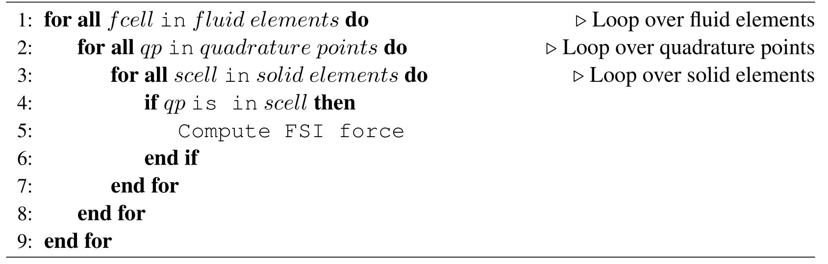
Algorithm 3.1 The nested searching loop for computing fluid FSI force

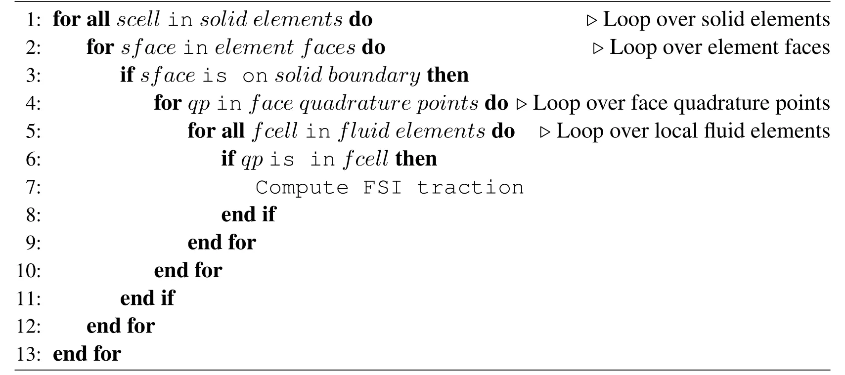
Algorithm 3.2 The nested searching loop for computing solid FSI traction

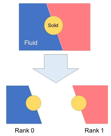
Figure 5:Combination of distributed mesh and shared mesh for FSI coupling

3.6 Adaptive mesh refinement

Adaptive mesh refinement(AMR)is widely used in fluid mechanics and solid mechanics simulations.It has become a component in many software packages,such as OpenFOAM[Greenshields (2015)] and ABAQUS [Smith (2014)].In FSI simulations,AMR has been used in ALE methods,as reported in Bathe et al.[Bathe and Zhang (2009);Boman and Ponthot (2012)],which are focused on preserving geometrical features at the interface.Feature reserving method is complicated as each type of nodes (corner,edge,surface and volume) must be treated with a different algorithm.In immersed methods,the major concern is that the fluid-structure interface projected from the solid is not explicitly represented but rather fitted into the background elements.If the background resolution is sufficiently fine,then the immersed solid has a sharper representation.If it is coarse,then the solid boundary is smeared.A mesh smoothing algorithm specialized for tetrahedral elements is implemented in Van Loon et al.[Van Loon,Anderson,De Hart et al.(2004)]for fictitious domain method,where the fluid elements that coincide with the solid boundaries are refined at every time step.In this smoothing method,the fluid nodes that lie on solid boundary must stay unchanged,therefore the number of nodes on solid boundary cannot be changed,which is a limitation on the resolution of the interface.On the other hand,a structural adaptive mesh refinement strategy is introduced[Vanella,Rabenold and Balaras(2010)] where block-structured rectangular patch grids are used,and embedded in the projection method to solve fluid governing equations.Similarly,AMR is implemented as a hierarchical structured Cartesian grids organized as a sequence of patches in Grifftith et al.[Griffith,Luo,Griffith et al.(2017)],where the target of the refinement is also the fluid-structure interface.This AMR method is designed specifically for structured grid,in which the neighborhood relationships are defined by storage arrangement.Therefore,it is suitable for finite difference method,but not for finite element method where the geometry is often too complicated to be meshed with structured grid.The AMR functionality in OpenIFEM is powered by p4est.p4est represents the grid as a quad/oct-tree of elements with different refinement levels,which is designed to work in parallel and scales to hundreds of thousands of processor cores.Different from the methods mentioned before,p4est works with unstructured quadrilateral and hexahedral elements,which can deal with complicated geometries.Also,as a mesh management tool designed for parallel computations,p4est supports additional functionalities such as mesh partitioning and ghosting.

Although p4est implements the mesh adaption algorithm which is ready to be used,two issues remain for user applications:1.the so-called hanging-node constraints;2.refinement/coarsening criterion.As illustrated in Fig.6,Q1andQ2denote two unrefined elements.Let us supposeQ2is refined once,which then split into 4 smaller elements;andQ3denotes the upper left one.Assuming each vertex is associated with one degree of freedom,and the IDs of the degrees of freedom along the edge betweenQ1,Q2arex0,x2,x1respectively.

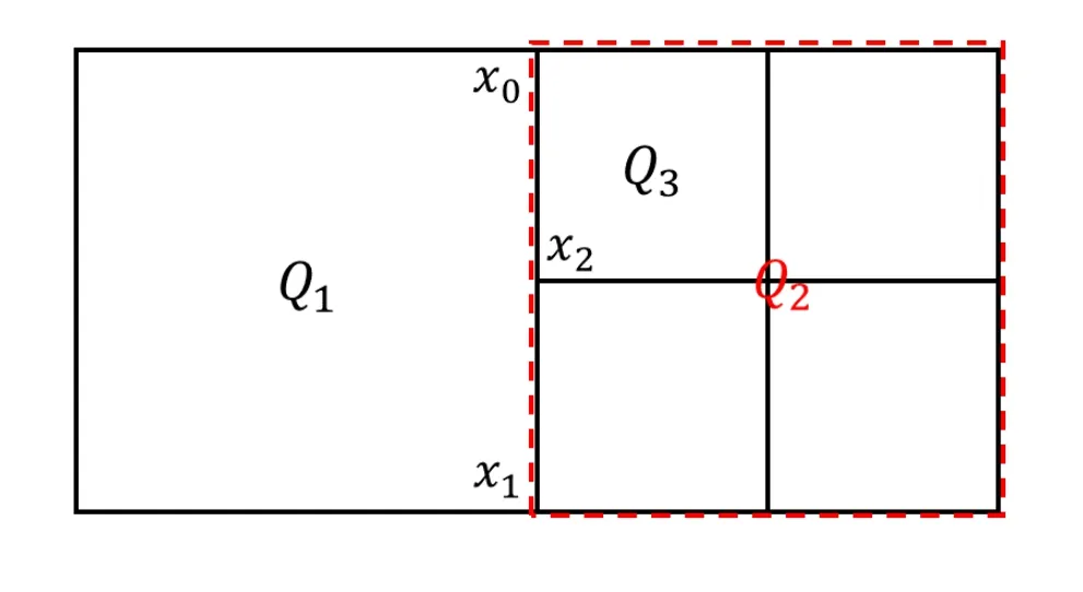
Figure 6:Illustration of hanging-node constraints

x2is not a degree of freedom inQ1,but the midpoint at the edge betweenx0andx1,it has to meet the following constraint:

This additional constraints due to the local refinement is called hanging-node constraints.As the mesh being refined or coarsened,hanging-node constraints are introduced into the system,on top of the regular constraints due to boundary conditions.As a result,the hanging-node constraints must be handled by the user application that utilizes p4est.In OpenIFEM,every time the mesh changes,initialize_system is called,in which the hanging-node constraints will be identified and added into the system constraints.The handling of hanging-node constraints is done through the interface of deal.II.

OpenIFEM defines two types of refinement/coarsening criterion.The first type is solution gradient based,which is used in fluid dynamics and solid mechanics computations.This method is proposed in Kelly et al.[Kelly,De SR Gago,Zienkiewicz et al.(1983)],where the jump of the solution (second derivative of solution) is evaluated at element faces and scaled by the size of element:

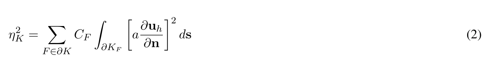
whereηKis the error estimator of elementK,∂Kis the boundary of elementK,∂KFis a particular faceFof elementK,CFandaare element size related parameters,is gradient of the solution,and [·] denotes the jump of a variable at a face.In independent fluid or solid simulations,the solution jumps are computed on all faces,and the elements with high jumps are refnied,and those with low jumps are coarsened.

The second refinement/coarsening type is location-based,similar to Griffith et al.[Griffith,Luo,Griffith et al.(2017)].In FSI applications,the location of interest is the fluid-structure interface which can be identified.In location-based strategy,an element is refined if it is close to the fluid-structure interface,and coarsened when it is further away from the interface.

wherePfis the center position of the fluid element under consideration,andPsis the center position of any solid element.hsis the solid mesh size,andChsis mesh-related parameter,which controls how large the refined region should be,which typically ranges from 1 to 10.

3.7 Cross-platform build system

Since OpenIFEM requires a number of dependencies to build,building and linking all the packages and libraries are complicated and tedious.It can be even more difficult to build the entire system on different types of platforms and environments,e.g.,Windows,Mac OS,Linux.CMake[Kitware Inc(2018)]provides a simple solution to put the pieces together without caring about the platform differences.CMake searches all the dependencies and verifies the version requirement,it then creates a makefile that can be used to build OpenIFEM library as well as test cases.After the library is built,it can be easily linked to other programs with CMake.

3.8 Test suite

OpenIFEM has a variety of test cases to ensure its accuracy and avoid regressions.The test cases cover general benchmark cases and special functionalities(time/space-dependent boundary conditions,etc.).Users can also add their own tests using the ctest module in CMake.

Adding a testTo add a test,a user can put a new test case file and its corresponding input file into a new directory in the tests directory using same name as the test case.Then the user should add the name of the test case into the test list in tests/CMakeLists.txt.After OpenIFEM is built,the new test case is automatically compiled.

Running a testTo run the tests,a user can simply use the command ctest to run all the test cases.To run only a specified subset of tests,the user can use argument-R followed by a string.All the test cases with names containing that string will be executed.More options can be found in CMake documentations[Kitware Inc(2018)].

3.9 Documentation,license and contribution

All the source code in OpenIFEM is well-documented,in a consistent style.Especially,the formulas used in the code are carefully explained so they can be easily understood.Doxygen is used to extract those comments and render them as pdf or html documents.OpenIFEM is under Apache License 2.0.The source code is free to access on https://github.com/OpenIFEM/OpenIFEM.We welcome contributions from the computational community and are open to issues and pull requests.

4 Numerical examples

OpenIFEM can be used to perform independent solid mechanics simulations,independent fluid mechanics simulations,and coupled FSI simulations.In this section,4 numerical simulation cases are presented to validate the solid solver,fluid solver and FSI solver in OpenIFEM,by comparing to analytical or other known numerical solutions.They are also included in the test suites.

4.1 Solid mechanics module

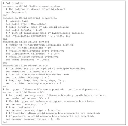
To validate the solid module,we perform a transient analysis on the bending of a 2D cantilever beam made of Neo-Hookean material.As shown in Fig.7,the cantilever beam is fixed on the left side,with a constant traction applied to the upper boundary.The length of the beam isL= 10 cm,the thickness isH= 1 cm.The material properties are shear modulesG= 5.955×105dyne/cm2,bulk modulusκ= 1×106dyne/cm2,densityρ= 1100 g/cm3.The imposed traction isT= 25 dyne/cm2along the entire length of the beam throughout the simulation time of 50 s.The time step used in this case is ∆t=0.1 s.A total of 640 uniform first-order quadrilateral elements are used and the number of degrees of freedom is 5120.The related parameters are shown in the following snippet of input file.

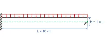
Figure 7:Setup of the cantilever beam test case.

The cantilever beam is initially at rest.The results are validated by comparing to ABAQUS[Smith(2014)].PointPdenotes the midpoint of the free boundary on the right,as shown in Fig.7.Fig.8 presents the profile of the vertical displacement atP.With the perturbed loading,the beam would initially bend downward reaching a maximum deflection of 5.1×10−1cm,until the external work equals the elastic energy.The inertia then takes the beam back to its original position with a small deflection of 3.0e−5cm.Without any damping,the beam bounces back and forth throughout the transient simulation period.The external work from loading is very small comparing to the elastic energy of the beam,resulting in small displacements at the equilibrium when the beam bounces back to its original position.

Figure 8:Vertical displacement of Point P over time

The deflection of the beam (indicated as the dashed line in Fig.7) att= 9 s,when the deflection is at its maximum,is plotted in Fig.9.The spatial distribution is highly nonlinear.The results obtained by OpenIFEM agree with ABAQUS perfectly.

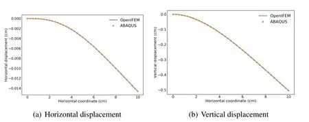
Figure 9:Displacement components on the centerline

4.2 Fluid mechanics module

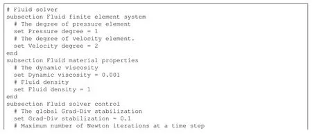
The fluid module is benchmarked with a 2D flow around a cylinder case at Reynolds number of 100 presented in [Schäfer,Turek,Durst et al.(1996)].Flow past a cylinder is a standard benchmark problem in many experimental and numerical studies,for example[Norberg(1994);Justesen(1991);Finn(1953)].As illustrated in Figure 10,a 2.2 cm long 0.41 cm wide rectangular fluid domain is modeled with a parabolic velocity boundary condition on the left boundary withVmax= 1.5 cm/s at the centerline.No-slip wall boundary conditions are applied to the upper and lower boundaries.A cylinder is placed at an offset of 0.01 cm lower than the centerline.The distance from the inlet to the center of the cylinder isLin= 0.2 cm,and the diameter of the cylinder isD= 0.1 cm.The fluid dynamic viscosity isµ= 0.001g/(cm·s) and the density isρ= 1 g/cm3.With a mean velocity of 1.0 cm/s,corresponding Reynolds number isRe= 100.The fluid solver parameter settings are specified in the following snippet of the input file:

The imposed input velocity is a function of they-coordinate,which is specified as a user-defined function in the test script,then passed onto the fluid solver.The following code snippet shows the declaration of the velocity boundary condition.

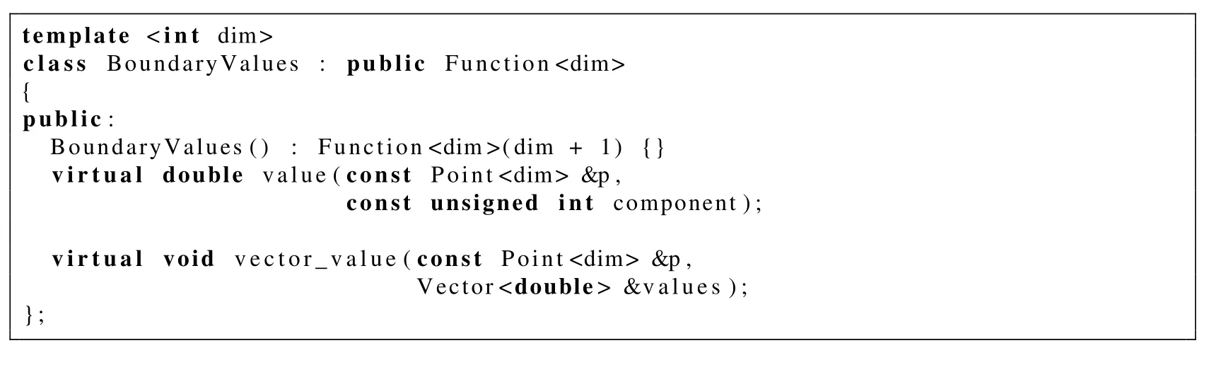
Figure 10:Setup of the flow around a cylinder test case

The mesh contains 5888 second order quadrilateral elements and 54192 degrees of freedom.The total simulation time is set to bet= 8 s to allow the flow to be fully developed.The time step used is ∆t=0.01s.

At this Reynolds number,the flow exhibits a periodic behavior with a vortex shedding behind the cylinder.The flow is fully-developed and the vortex shedding becomes periodic aftert= 4 s.Fig.11 shows the velocity and pressure fields att= 8 s,where the vortices can be clearly seen.

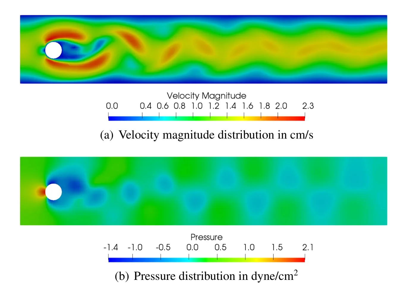
Figure 11:Velocity magnitude and pressure distributions at t=8 s

To verify the results quantitatively,the drag coefficientCDand lift coefficientCLof the cylindrical wall are evaluated using:

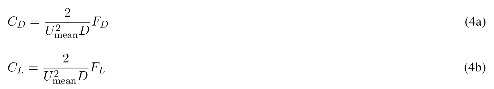
whereFDandFLare the drag and lift forces respectively,andUmeandenotes the mean velocity at the inlet andDis the diameter of the cylinder.

Fig.12 shows the drag and lift coefficients over time,where the average drag coefficient is found to beCD= 2.19,very close to the experimental result 2.05 in Finn[Finn(1953)].The frequency is found to bef= 3.01 Hz and lift coefficient amplitude is|CL|= 1.00,which are also in good agreement with schafer et al.[Schäfer,Turek,Durst et al.(1996)].

4.3 FSI module

We present 2 numerical examples for the FSI module,one is free fall of an almost rigid solid body,the second one is a soft solid with large deformation.Similar problems are analyzed with original and modified IFEM algorithm in Zhang et al.[Zhang and Gay(2007);Wang and Zhang (2013)],where the free fall of a rigid cylinder can be compared to empirical solutions.

4.3.1 Free falling of a 2D disk

In this example,a 2D disk falls in the viscous fluid driven by gravityg=980 cm/s2.The disk is modeled with Neo-Hookean material that has large shear (G=3.36×106dyne/cm2)and bulk moduli(κ= 8.33×107dyne/cm2),close to a rigid body.The solid density isρs= 2.6 g/cm3.The fluid dynamics viscosity isµ= 1g/(cm·s)and density isρf= 1 g/cm3.The height of the computational domainH= 6 cm,width of domainW= 2 cm,diameter of the diskD= 0.25 cm.The left,lower and right boundaries of the fluid domain are modeled as no-slip walls,the upper boundary is a no-penetration boundary.The initial position of the disk is at the vertical centerline of the fluid domain,with a distanceh= 1 cm from the upper boundary.The setup is shown in Figure 13.The system is solved with a time step of ∆t= 0.001 s.The definition of material properties in the input file is similar to the previous cases,therefore we show a snippet of the“Simulation”section in the input file where the simulation type is specified as“FSI”.

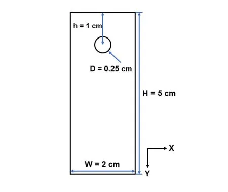
Figure 13:Setup of the free falling of 2D disk test case

The vertical velocity of the center of the disk over time is shown in Fig.14.The solid disk falls with increasing velocity that is driven by gravity.Due to the drag of the viscous fluid,the acceleration gradually decreases until the drag and the body forces are balanced,which allows the disk to reach a terminal velocity of 7.33 cm/s.Eq.(5)is an empirical formula compiled from experimental results given by Clift et al.[Clift,Grace and Weber(2005)].ρsandρfdenote the densities of the solid and the fluid,respectively;µis the fluid dynamic viscosity;Ris the radius of the disk,andWis the width of the fluid domain.The ratio betweenWandRreflects the wall effect.As the fluid domain becomes wider,lnterm becomes dominant.Comparing to terminal velocity of 7.29 cm/s yielded from the empirical formula,the discrepancy in terminal velocities between the simulated one and empirical one is only 0.55%.

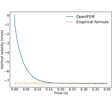
Figure 14:Vertical velocity of the disk vs.time.

We also examine the velocity distributions in Fig.15.From the horizontal velocity (vx)distributions(a-c),we can see that as the disk falls downward,it pushes the upstream fluid to both sides.In the downstream,the horizontal velocity shows an opposite pattern,where the fluid on both sides moves toward the center,forming two vortices.Thevxcontour shows the outlines of the high and low velocity regions.At the beginning,the velocity contours in the upstream and downstream regions have similar shapes;as the disk falls,the contours in the downstream stretch out while the contours in the upstream do not.This is due to the fact that the upstream fluid is always in touch with the disk,but the high velocity in the downstream fluid is diffused by the viscosity after the disk moves away.

The vertical velocity,vy,has a different pattern(d-f).The minimumvy(maximum velocity in the direction of gravity) occurs in the surrounding area of the disk,and propagates to the adjacent region.Symmetrically large positivevyis observed in the near wall regions.Similar tovx,the velocity contours in the downstream is gradually stretched out by viscosity.The velocity patterns agree very well with solutions reported in Lee et al.[Lee,Chang,Choi et al.(2008);Zhang,Liu and Khoo(2012)].

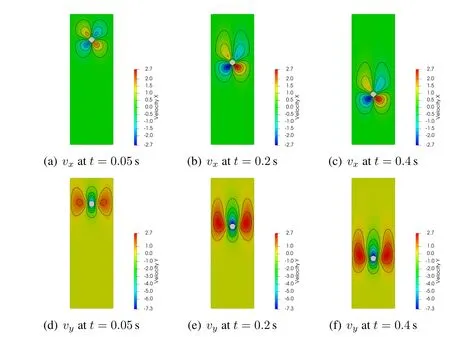
Figure 15:Velocity distributions and contours in cm/s at different time

To examine the fluid near the disk,Fig.16 shows the zoomed-in view of the velocity vectors and the pressure contours.From the velocity vector plot we can clearly see two symmetric vortices behind the disk.Due to the hydrostatic pressure,the pressure distribution is almost linear except near the body of the disk where the pressure on the lower part of the disk surface is higher than the surrounding fluid while the upper part is smaller.This observation also agrees with the results obtained by other numerical models [Zhang,Liu and Khoo(2012);Banks,Henshaw,Schwendeman et al.(2017a,b)].

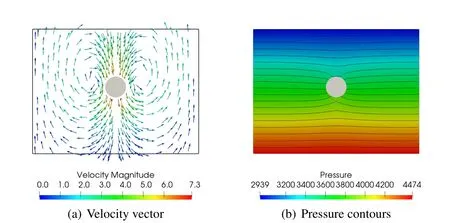
Figure 16:Zoomed-in velocity in cm/s and pressure distributions in dyne/cm2 at t=0.4s

4.3.2 Large deformation of a leaflet driven by incompressible flow

Finally,we present an FSI case where the solid deformation is largely driven by an incoming flow.As illustrated in Fig.17,a leaflet is fixed at the bottom of a rectangular fluid domain sized 1 cm×4 cm,and placed 1 cm from the left boundary of the fluid domain.The width of the solid is 0.1 cm and the height is 0.4 cm.The material is modeled as nearly incompressible Neo-Hookean with a shear modulus ofG= 7×104dyne/cm2and a bulk modulus ofκ= 8.6×106dyne/cm2,which corresponding to an initial Young’s modulus of 1.9×105dyne/cm2and Poisson’s ratio of 0.49.The solid density is set toρs=6 g/cm3.The width of the fluid domain is 4 cm and height is 1 cm.The fluid density isρf=1 g/cm3and the dynamic viscosity isµ= 0.1g/(cm·s).Constant velocity inputV0= 25 cm/s is specified on the left boundary of the fluid domain,the bottom boundary is modeled as no-slip wall,while the upper boundary has no-penetration condition,and the right boundary is outflow.The Reynolds number is 250.This relatively high incoming velocity is challenging to traditional immersed approach because the solid displacement would likely be overestimated[Wang and Zhang(2013)]as the solid displacement is evaluated using the fluid velocity.

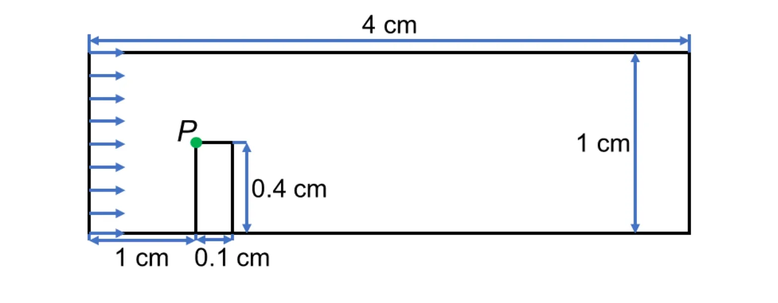
Figure 17:Setup of the leaflet case

There are 2200 second order quadrilateral fluid elements with 20533 degrees of freedom,as well as 256 first order quadrilateral solid elements with 2048 degrees of freedom used.The time step is set to be ∆t= 5e−4s.The simulation is run for 0.2swhen the steady state is obtained.The displacement magnitude of the upper left corner of the leafletP,marked as green dot in Fig.17 is monitored.As can be seen in Fig.18,as the flow begins to develop,PointPundergoes a large displacement 5 times that of the height of the leaflet.Then the leaflet starts to vibrate,but with decreasing amplitude.The displacement of PointPfinally stabilizes at 0.1s,converging to 0.105cm.The boundary conditions in this case are specified in the input file,which is listed in the following snippet:

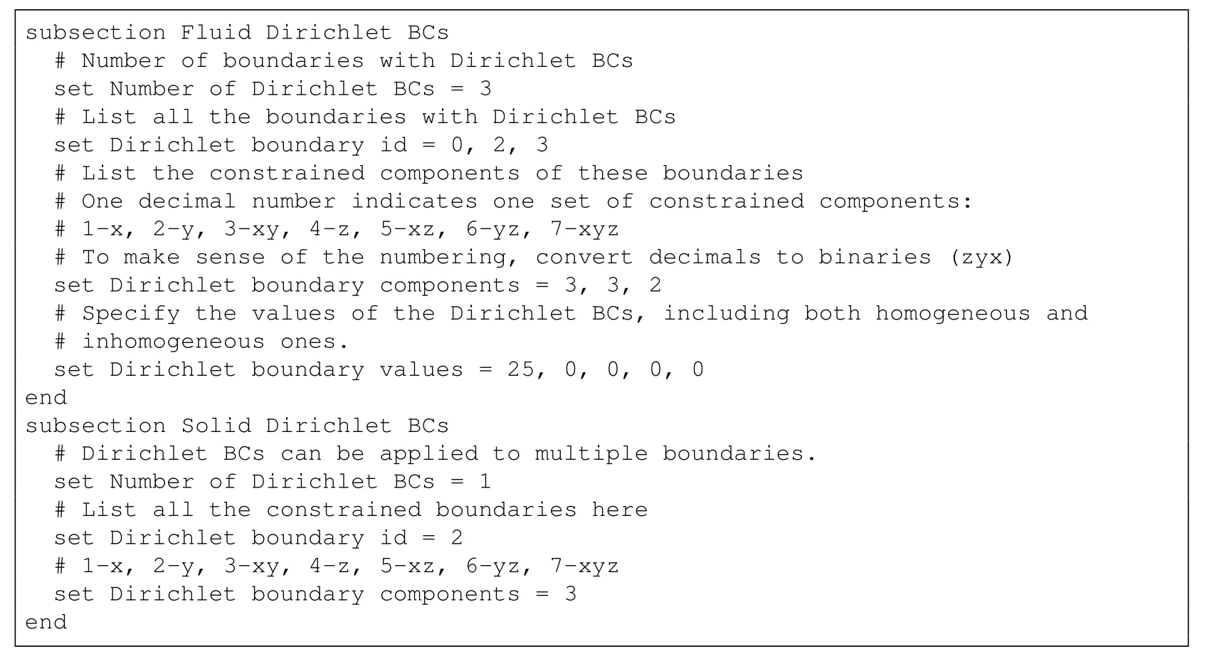
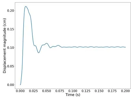
Figure 18:Displacement magnitude of Point P.

We show the fluid velocity at four different times in Fig.19.The deformation of the solid is very significant,but the volume is still conserved.In fact,by integrating the JacobianJat the quadrature points,the volume change of the solid is less than 0.1%.In addition,a large velocity gradient area is observed near the upper left corner of the leaflet,which produces large vortices in the downstream.Att= 0.2 s the fluid field is fully developed and the solid oscillation has stopped,where the upper part is dominated by high velocity flow,and the velocity in the lower part is much smaller.

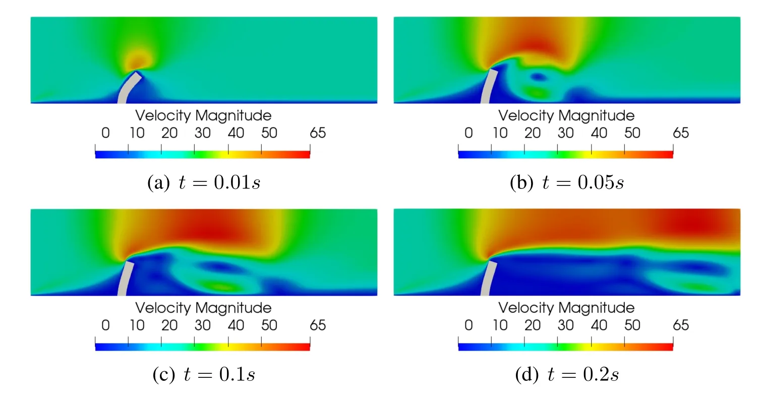
Figure 19:Velocity magnitude in cm/s with contours at different time

Correspondingly,the pressure field is shown in Fig.20.A sharp jump near the solid is identified due to the existence of the solid.A negative pressure region representing flow recirculation is formed and shed from the tip of the leaflet.A similar numerical example with large deformation is studied in Zhang et al.[Zhang,Liu and Khoo(2012)],in which same flow pattern is obtained.

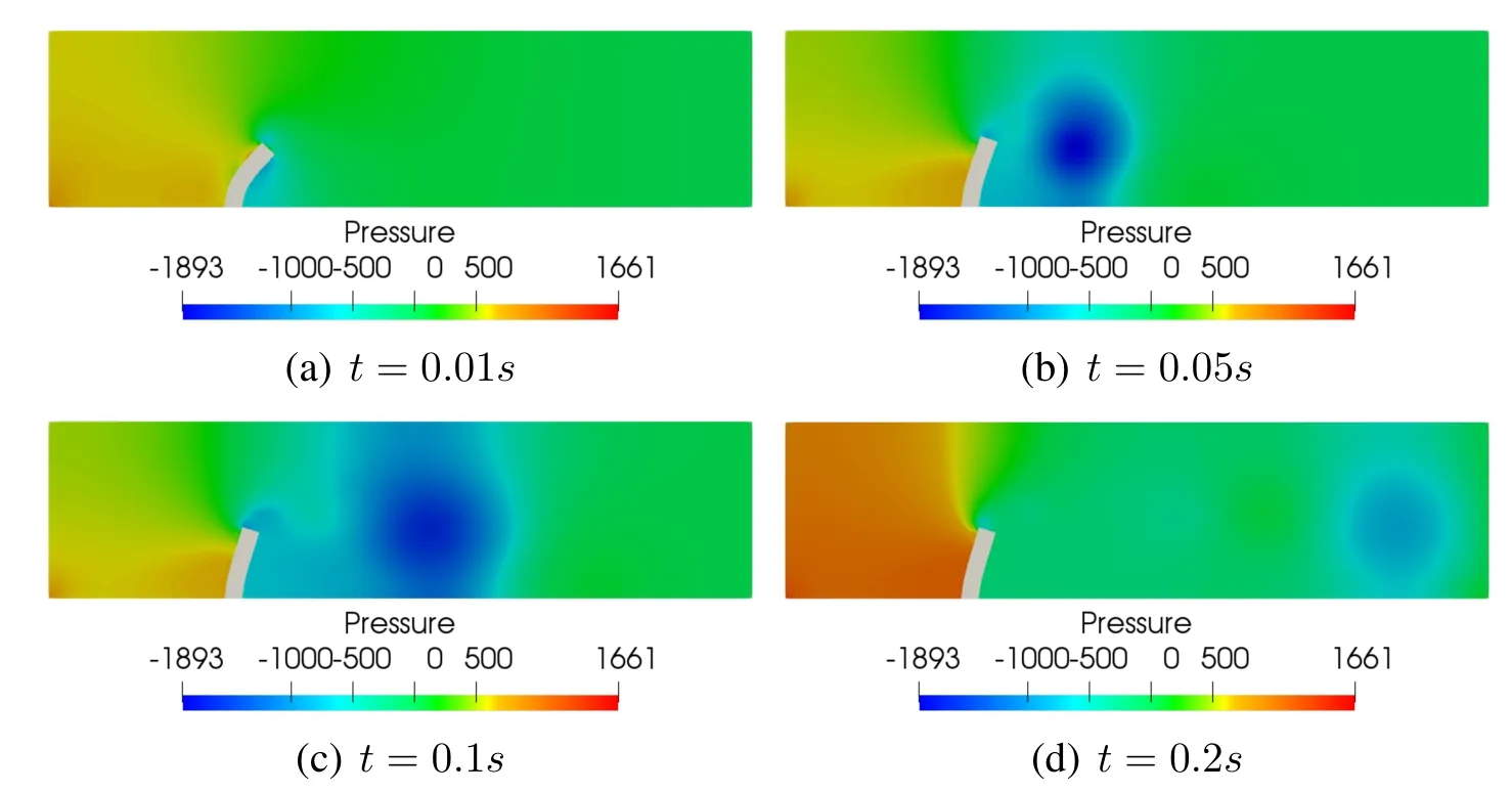
Figure 20:Pressure field in dyne/cm2 at different time

5 Conclusions

In this paper,we present a high performance modularly built open-source software,the OpenIFEM,for FSI problems.It is the first comprehensive software package focused on solving FSI problems using modular components,i.e.,independent Eulerian and Lagrangian solvers,which fills the void in this field.The code is written in object-oriented way,with modern design that allows easy customization.Many basic building blocks in finite element programming and linear algebra are handled by third-party libraries,which significantly reduces the size of the code base and improves the maintainability.Four numerical examples are presented to verify the solvers in the solid,fluid and FSI modules of OpenIFEM.More testing problems in 2D and 3D can be found online.Comparing to other immersed method packages,OpenIFEM has modularity,extensibility,flexibility,maintainability,efficient parallel implementation,test suites and thorough documentation.We expect this project to be helpful to other researchers in this area and welcome contributions from the community.

Acknowledgement:Author Lucy T.Zhang would like to thank NSFC 11550110185,NSFC 11650410650,and NIH-2R01DC005642-10A1 for funding support.