An Immersed Method Based on Cut-Cells for the Simulation of 2D Incompressible Fluid Flows Past Solid Structures

François Bouchon ,Thierry Dubois and Nicolas James

1 Université Clermont Auvergne,CNRS,LMBP,F-63000 CLERMONT-FERRAND,France.

3 Laboratoire de Mathématiques et Applications UMR 7348,Université de Poitiers,Téléport 2 -B.P.30179,Boulevard Marie et Pierre Curie,86962 Futuroscope Chasseneuil Cedex,France.

Abstract: We present a cut-cell method for the simulation of 2D incompressible flows past obstacles.It consists in using the MAC scheme on cartesian grids and imposing Dirchlet boundary conditions for the velocity field on the boundary of solid structures following the Shortley-Weller formulation.In order to ensure local conservation properties,viscous and convecting terms are discretized in a finite volume way.The scheme is second order implicit in time for the linear part,the linear systems are solved by the use of the capacitance matrix method for non-moving obstacles.Numerical results of flows around an impulsively started circular cylinder are presented which confirm the efficiency of the method,for Reynolds numbers 1000 and 3000.An example of flows around a moving rigid body at Reynolds number 800 is also shown,a solver using the PETSc-Library has been prefered in this context to solve the linear systems.

Keywords:Immersed boundary methods,cutt-cell methods,incompressible viscous flows.

1 Introduction

For some decades,many researchers and engineers have been considering the numerical solution of fluid flows,for different kind of fluids and different geometries.With the increasing performance of super-computers,it has been possible to tackle more and more challenging problems,for higher Reynolds numbers and complex geometries.Several different discretization techniques can be used to consider these problems:Finite Element Methods,Finite Volumes Methods,Spectral Methods,and Finite Difference Methods.The MAC scheme on cartesian grids[Harlow and Welch(1965)]can be viewed both as a Finite Volume Method or a Finite Difference Method on staggered grids,and is adapted to 2D or 3D flows in simple geometries,for example for lid-driven cavity or backward facing step.To take into account some obstacles in the flows(or complex geometries),immersed boundary techniques have been developped by Peskin in the 80’s [Peskin (1982,2002)],consisting in using Dirac functions to model the interacting force between the fluid and the solid structure.These methods have inspired many authors in the following years,Mohd-Yusof has combined them with the use of B-Splines [Mohd-Yusof (1997)] in his momentum forcing methods to consider complex geometries.The main advantage of these techniques is that the forcing term does not change the spatial operators,making them quite easy to implement(see Mittal et al.[Mittal and Iaccarino(2005)]for a review,and refences therein).As an alternative,Bruno et al.have developped penalization techniques to inforce suitable boundary conditions[Angot,Bruneau and Fabrie(1999)].Similar techniques have also been investigated by Maury et al.[Janela,Lefebvre and Maury(2005)]and justified from a mathematical point of view in Maury [Maury (2009)].These methods have been shown to be efficient in the context of several particles in a flow [Lefebvre (2007)],and when considering possible collisions between them[Verdon,Lefebvre-Lepot,Lobry et al.(2010)].

Arbitrary Lagrangian Eulerian (ALE) methods have been developped for flows in geometries which vary in time (see Richter et al.[Richter (2013,2015);Yang,Richter,Jager et al.(2016)]where authors use some of the ideas of[Belytschko(1980)]).The aim is to formulate the equation in a fixed reference domain,by using a mapping from the reference domain Ω(0)to the domain Ω(t)occupied by the fluid at timet.The position of the moving bodies,which correspond to the boundary of Ω(t),being available,the velocity field of these bodies defined on∂Ω(t) have to be extended to Ω(t).Once this is done(generally with harmonic extensions),the equations are written in the reference domain by using the chain-rule formula.

For problems involving non-rigid bodies,Roshchenko et al.[Roshchenko,Minev and Finlayb(2015)]have used splitting methods to solve first the evolution of the velocity field in the fluid,and then to consider the deformation of the body.These ideas of splitting the model can be viewed as similar to the projection techniques(see Chorin[Chorin(1968)],and Guermond et al.[Guermond,Minev and Shen (2006)] for a review and references therein).

The method presented in this work joints another family of methods,called cut-cell methods.The idea of these methods is to modify the discretization of the Navier-Stokes Equations in the cells cut by the immersed boundary[Ye,Mittal,Udaykumar et al.(1999);Mittal,Dong,Bozkurttas et al.(2008);Tucker and Pan (2000);Chung (2006)].One can discretize the equations on smallest cells obtained by intersecting the grid-cell with the domain occupied by the fluid,or one can merge these smallest cells with a neighbouring one.These methods can be combined with the levelset methods to track the boundary of the fixed or moving body[Osher and Sethian(1988).These ideas are used in the present work:the body in the fluid is represented by a levelset function,and the location of the velocity components are modified in the cut-cells [Bouchon,Dubois and James (2012)],the pressure remaining placed at the center of cartesian grid cells for both fluid-cells and cut-cells.For the Laplacian of the velocity,the classical five-point approximation must be replaced by a local 6-point formula,for which the truncation error is only first order.But as in Matsunage et al.[Matsunaga and Yamamoto(2000)],global second order convergence of the method is recovered.This second-order convergence for the velocity and the pressure with our cut-cell scheme has been obtained for the flow past a circular cylinder at Re=40 in James et al.[James,Biau,Dambrine et al.(2013)] by comparing with the reference solution proposed in[Gautier,Biau and Lamballais(2013)].

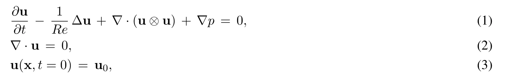
Figure 1:The solid body ΩS with boundary ΓS and the surrounding computational domainΩF in which the flow is to be simulated

The paper is organized as follows:Section 2 is devoted to the presentation of the problem.The Navier-Stokes Equations are considered in a 2D geometry,which is supposed to be fixed for the sake of c larity.We also introduce there the notation for the grids,and detail space discretization.In Section 3,we give some information about computational aspects.In the case of fixed d omain,a fast s olver a dapted f rom t he c apacitance m atrix method [Buzbee,Dorr,George et al.(1971);Buzbee and Dorr (1974)] is used to solve the linear systems for both components and for the pressure.We also show that the method can be adapted in the case of moving domain.In this context,the preprocessing step of the capacitance matrix method would need to be done at each time-iteration which would then increase the CPU time.Therefore,we have prefered for this case a parallel version of an algebraic multigrid method (HYPRE BoomerAMG) implemented using the PETSc Fortran library [Balay,Abhyankar,Adams et al.(2018a,b)].

Section 4 is then devoted to numerical tests,where we compare our results with theoretical predictions and other numerical results available in the literature.A conclusion is given in Section 5.

2 The setting of the problem

2.1 Flows past obstacles

We consider a flow in a two-dimensional domain Ω = (0,L)×(0,H) which contains a domain ΩSoccupied by the solid which is supposed to be fixed for the sake of simplicity.We denote then ΩF=ΩΩSthe domain occupied by the fluid(Fig.1).

The velocity field in the fluid satisfies the Navier-Stokes equations,with no-slip boundary conditions.We consider then the problem:

where u(x,t) = (u,v) is the velocity field at x = (x,y)∈ΩFat timet >0,u0is the initial condition andReis the Reynolds number.We impose homogeneous Dirichlet boundary conditions for the velocity field on∂ΩF:

We mention that non-homogenous Dirichlet boundary conditions can also be treated with the method presented here.

2.2 Discretization

For the time-discretization of(1)-(3),we use a second-order backward difference(BDF2)projection scheme.In a first step,the velocity field is advanced in time with a semi-implicit scheme decoupling the velocity and pressure unknowns.Then,the intermediate velocity is projected in order to obtain a free-divergence velocity field.

Letδt >0 stand for the time step andtk=k δtdiscrete time values.Let us consider that(uj,Pj)are known forj ≤k.The computation of(uk+1,Pk+1)needs two steps:

with homogeneous Dirichlet boundary condition for

Then the intermediate velocity fieldis projected in the free-divergence space to get

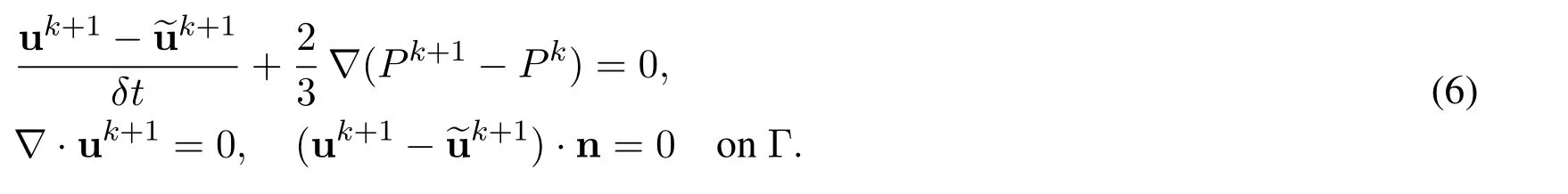
For the spatial discretization,we modify the MAC scheme near the boundary by changing the location of the unknowns of the velocity components for the cells cut by the solid as depicted on Fig.2,the pressure unknowns remaining in their original place(see[Bouchon,Dubois and James (2012)] for more details).To discretize the Laplacian in (5),we must replace the five-point formula by a six-point discretization.For the convective terms,the fluxes are computed at the midle of the vertical and horizontal edges (see Fig.3).For the pressure,linear interpolation are used rather than changing the location of the pressure unknowns.The same kind of linear interpolation is used to get consistant evaluation of the pressure gradient in(6).

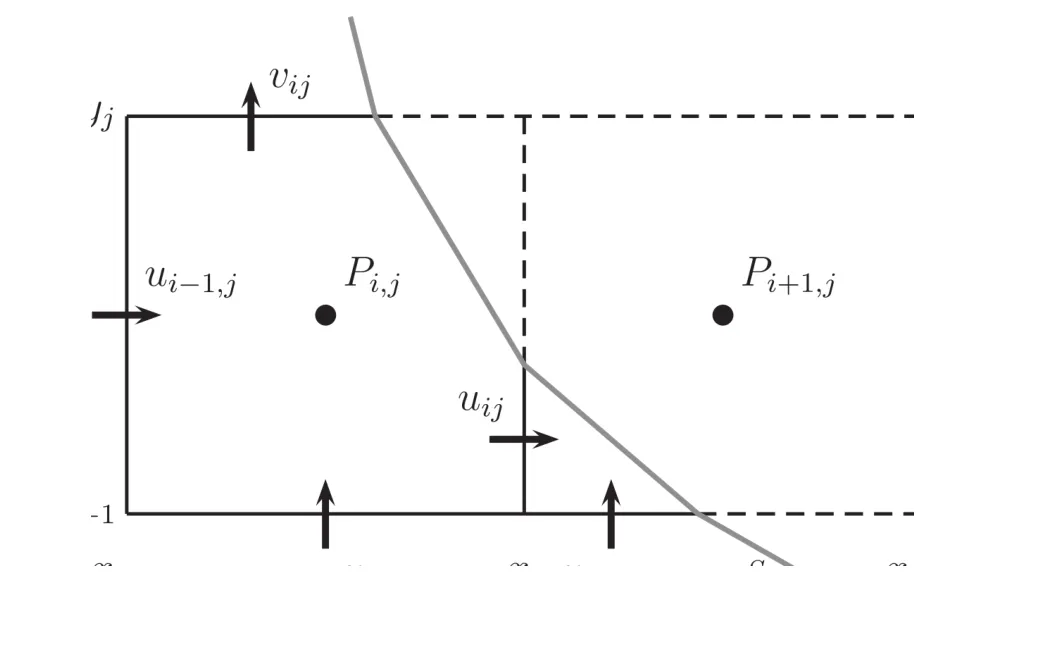
Figure 2:Location of the unknowns near the solid body

Figure 3:Location of the computation of the fluxes near the solid body

Although the truncation error is only first order in space for the resulting numerical scheme,the second order accuracy is recovered which is due to a superconvergence phenomena analoguous to those proven in Matsunaga et al.[Matsunaga and Yamamoto(2000)].This second order has been observed in James et al.[James,Biau,Dambrine et al.(2013)]by showing results in comparison with those of Gautier et al.[Gautier,Biau and Lamballais(2013)].

3 Computational aspects

3.1 A fast parallel direct solver to treat fixed solid strutures

When considering fixed solid bodies,the use of a direct solver with a preprocessing procedure is efficient.Once the preprocessing computations have been done,the cost paid to solve the linear systems is about twice the case of a numerical simulation in the same computational domain without obstacles.We summarize hereafter the fast direct solver derived from the capacitance matrix method and adapted to the case of non uniform grids[Bouchon,Dubois and James(2012);Bouchon and Peichl(2010)]for the details which has been implemented in our code.

After spatial discretization of the Navier-Stokes equations,one linear equation is obtained per node in the part of the computational domain filled by the fluid and per unknown that isu,vandp.We complete these sets of linear equations by adding similar ones for nodes of the cartesian grid lying inside the solid obstacle but with zero as right-hand side.The unknowns corresponding to mesh points in ΩShare fictitious ones.As in ΩF,the numerical scheme accounts for the boundary conditions on ΓSh,the fluid unknowns are independant to the solid ones.We therefore obtain linear algebraic systems defined on the whole cartesian grid withnx×nymesh points whose sizes are(nx−1)×nyforu,nx×(ny−1)forvand(nx−1)×(ny−1)forp.All three linear systems are similar in nature:the resulting matrices have similar structures with five or six non-zero coefficients per row.

Let us consider one of these linear system.We denote byNits size and byA ∈MN(R)its matrix.Then at each time iteration,we have to solve a linear system

with the right-hand sideZcomputed from the velocity and the pressure at previous time steps.As it is mentioned above,the matrixAis non-symmetric.Let us consider now the matrixGobtained with the same discretization on the whole computational domainΩ totally filled by a fluid that is with no obstacles.The matricesAandGdiffer only on rows corresponding to computational meshes for which the five-point stencil interacts with a cut-cell.Let us denote byncthis total number of rows,namely rows such thatA−Ghave non-vanishing coefficients.The efficiency of our direct solver is due to the fact thatncis small compared withNand that the non-zero coefficients on each row ofA−Gis bounded.The linear system(7)can be rewritten as

whereQis a matrix of dimensionsN×ncwith one non-vanishing coefficient per column,equal to one,andY ∈Rncsuch that

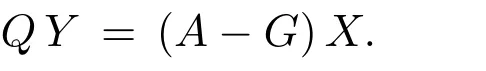
It can be easily shown,usingQtQ=Inc,thatYis solution of the following linear system

withM=Qt(A−G).The matrixInc+M G−1Qis a non-singular matrix(see Bouchon and Peichl(2010)for a proof)of sizenc.

Based on these relations,the algorithm implemented to solve(7)consists in a preprocessing step where the matrixInc+M G−1Qis factorized(we use aLU-factorization)followed by

i) ComputeZand solveGW=Z;

ii) ComputeMWand solve(9);

iii) ComputeQYand solveGX=Z−QY.

Recalling thatGis the matrix corresponding to the standard MAC scheme on the whole computational mesh,steps i) and iii) can be performed by using any efficient solvers available on cartesian grids.In the present work,we use Discrete Fourier transforms in the vertical direction(where the mesh is uniform)combined withLU-factorizations of the resulting tridiagonal systems.

The parallel version of this direct solver is based on explicit communications performed by calling functions of the MPI library.The main feature of MPI is that a parallel application consists in runningpindependant processes which may be executed on different computers,processors or cores.These processes can exchange datas by sending/receiving messagesviaa network connecting all the involved computing units.

The first step when developping a parallel algorithm is to define a suitable and efficient splitting of the datas among the MPI processes:each MPI process will treat datas associated with a part of the total computational mesh.For our problem,this choice is straightforward and is related to the algorithm used to solve the linear systems.Indeed,it is much easier to implement a parallel resolution of tridiagonal linear systems rather than a parallel version of the DFT.Therefore,the parallel version of the code is based on a splitting of the datas along the horizontal axis,so that each MPI process works with a vertical slice of the computational mesh as it is illustrated on Fig.4.

In the framework of finite volume or finite difference schemes on cartesian grids,the explicit computation of spatial derivatives is local and involves very few communications.The only tricky part concerns the resolution of the linear systems.The step ii)of the direct solver described in the previous section consists in solving a linear system involving the matrixInc+M G−1Q.As theLU-factorization of this matrix has been computed and stored in a pre-processing step at the beginning of the time iterations,we have to solve two triangular systems which can not be efficiently performed on parallel computers.Asncis small compared to the size of the global problem,we choose to dedicate this task to one given MPI process (fixed in advance) per unknown,that isu,vandp.Once these linear systems are solved,the resulting vectors are scattered from these MPI processes to the other ones.

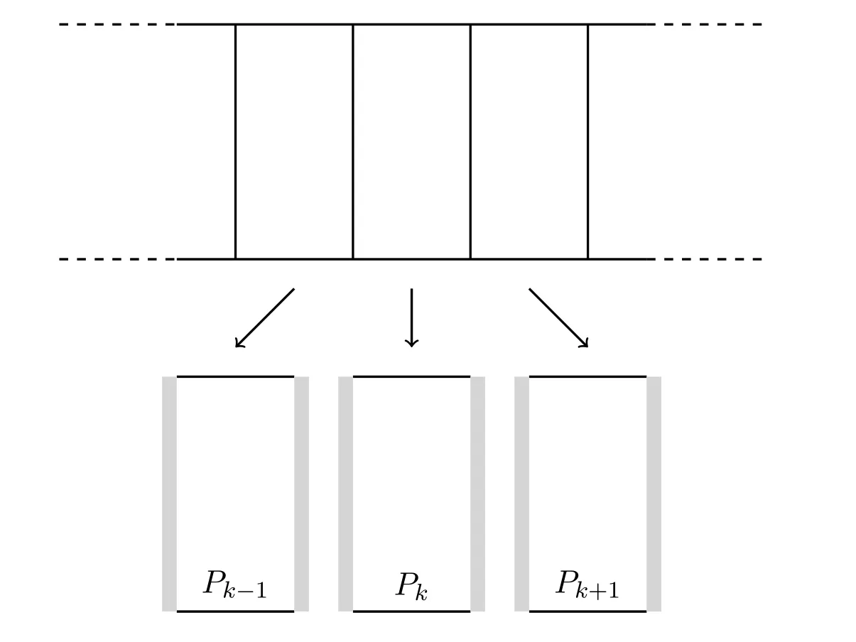
Figure 4:Splitting of the computational grid among the MPI processes Pk,k =0,...,p−1.The gray zone refers to additional (ghost points) storage used for the MPI communications between neighbooring processes

As it was previously mentioned,linear systems of steps i)and ii)are solved by first applying a DFT in they-direction:these computations are independant and can be performed without any communications due to the distribution of datas among the MPI processes.This results in a collection,one per grid point in they-direction,of independant tridiagonal linear systems connecting all nodes of the mesh in thex-direction.A parallel direct solver based on thedivide and conquer approach(DAC)for tridiagonal matrices has been implemented[Bondeli (1991)].The DAC method,applied to solve one tridiagonal linear system onnp >1 MPI processes,consists in splitting the tridiagonal matrix intonpindependant blocks(one per MPI process).The solutions of these systems have to be corrected in order to recover the solution of the global system.These corrections correspond to 2np−1 values which are solutions of a tridiagonal linear system of size 2np−1.This phase of the DAC method is sequential and has to be performed on one process inducing a useless waiting time for the other processes.However,as we have to solvenysuch systems simultaneously,this sequential part can be distributed among all thenpprocesses.In this context,the DAC algorithm leads to an efficient parallel code.

The parallel code has a good level of performance:less than 15%of the CPU time is spent in communications between MPI processes.The sequential part performed on one process represents a negligible amount of CPU time.The computations presented here have been performed on a DELL cluster using up to 32 cores of Xeon processors.A low latency bandwith network connects the cluster nodes.

3.2 Iterative solver for the case of moving bodies

For solid bodies moving in a computational domain filled by a fluid,as the case considered in Section 4.2,cut-cells may change at each time iteration.Therefore,the coefficients of the matrices of the linear systems for the velocity components,issued from the discretizetion of the momentum equations,and for the pressure increment computed in the projection step of the time scheme,have to be recomputed at each time step.In that context,the use of the fast direct solver described in the previous section is cumbersome and inefficient except on coarse meshes.In order to be able to treat such configurations,we have implemented a PETSc version [Balay,Abhyankar,Adams et al.(2018a,b)] of our cut-cell scheme.The main advantage of the PETSc Library is that,in a parallel programming environment based on MPI,many iterative solvers combined with different preconditionners can be used.The choice can be made at run time.

4 Numerical results

4.1 Flow past a circular cylinder at Re=1000 and 3000

In this section,we present numerical simulations,performed with the parallel direct solver method described in Section 3.1.We consider the case of flows past a fixed circular cylinder of diameterD.The Reynolds number is defined based on the diameterDof the cylinder,i.e.,Re =U∞D/νwhereU∞is the horizontal free stream velocity.As non-dimensional time,we considerT=2U∞t/D.

A circular cylinder of diameter equals to unity is centered at the origin of the computational domain Ω = (−Lx,Lx)×(−Ly,Ly).As boundary conditions,a uniform velocity profile u(x =−Lx,t) = (1,0)is imposed at the inflow and a convective boundary condition is applied at the exit,namely the convective equation

is solved atx=Lx.On the top and bottom boundaries,that isy=±Ly,slip boundary conditions are used that is= 0 andv= 0.Finally,no-slip (u|ΓS= 0) boundary condition is applied on the surface of the obstacle.

For this problem important quantities reflecting the dynamics of the vortices formed in the vicinity of the solid boundary and developping at the rear of the cylinder are the pressure drag and lift coefficients.They are derived from the total drag force on the body,which is computed as

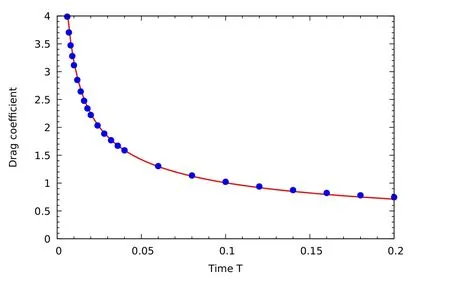
Figure 5:Evolution of the drag coefficient of a circular cylinder at Re = 1000.Solid line(red):theoretical prediction (12);Blue dots:numerical results on a 4096×8192 grid inΩ=(−10,10)2

The pressure drag and lift coefficientsandare given byCp= 2Fb ·exand=2Fb ·eyand the (total) drag coefficient isCd=Cp+.Starting with a flow at rest,the drag coefficient behaves asT−1/2in the early stage of the development of the vortices.This square-root singularity has been theoretically predicted by Bar-Lev et al.[Bar-Lev and Yang(1975)].They have derived the following expression for the(total)drag coefficient

As whown in Fig.5,the values obtained with the cut-cell scheme on a grid with 4096×8192 mesh points discretizing the domain Ω = (−10,10)2perfectly match the theoretical curve drawing(12)on the time intervalT ∈[0,0.2]for Re = 1000.Our cut-cell method captures the square-root singularity of the drag coefficient.This simulation has been run using 16 MPI processes.On longer time interval,namelyT ∈[0,5],the results are in good agreement with those obtained by Koumoutsakos and Leonard in Koumoutsakos et al.[Koumoutsakos and Leonard (1995)] with a vortex method.In order to test the grid convergence of these results,the same simulation has been conducted on a grid with two times more points in both spatial directions,that is 8192×16384 mesh points,in the same computational domain.In that case,32 MPI processes have been used.Both results are almost indistinguishable on Fig.6 indicating that the coarser resolution is enough to capture the essential features of the flow at this Reynolds number.The development of the flow around the impulsively started cylinder at Re = 1000 can be seen on Fig.7.In the early stageT ≤1,a primary vortex develops in the vinicity of the boundary at the rear of the cylinder.Then forT ∈[1,2]a secondary vortex appears trying to move insight the primary vortex and to push it away from the solid boundary(T ≥4).A tertiary vortex is visible atT=3 which remains sticked to the boundary constrained by the two other vortices having more strength.These results compare well with the same flow representations shown in Koumoutsakos et al.[Koumoutsakos and Leonard (1995)].As expected on short time interval(T ≤5)the flow remains symmetric.

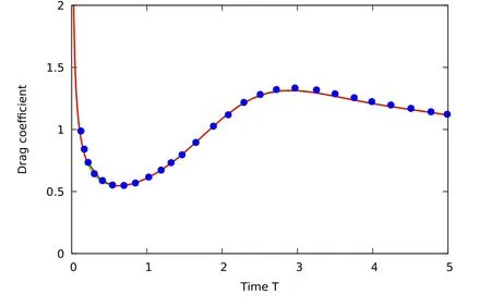
Figure 6:Evolution of the drag coefficient of a circular cylinder at Re = 1000.Red solid line:numerical results on a 4096 × 8192 grid in Ω = (−10,10)2;Green solid line:numerical results on a 8192 × 16384 grid in Ω = (−10,10)2;Blue dots:results from[Koumoutsakos and Leonard(1995)]

At Re = 3000,the time evolution of the drag coefficient plotted on Fig.8 exhibits also the square-root singularity on short time interval and is in good agreement with the results of Koumoutsakos and Leonard.As expected,the drag coefficients remains almost constant forT ∈[2,3] [Koumoutsakos and Leonard (1995)].Note that on this time interval,a small difference exists between the results computed on the two different grids.However,the coarser simulation is fine enough to capture the flow dynamics at Re = 3000.The mesh size of the coarser grid,which is constant in the vicinity of the solid boundary,ish= 20/8192≈2.44×10−3.Note that the size of the computational domain and the boundary conditions imposed at the exit may influence the results.Estimating the values forLxandLyrequired so that the numerical results being of the order of the numerical scheme error,namely O(h2),is an open question.This will be addressed in further works.At this Reynolds number,a scenario similar than that at Re = 1000 can be observed on Figure 9 with the development of three vortices in the early stage of the flow dynamics.The secondary vortex penetrates further inside the primary vortex aera and the tertiary vortex has more strength as it could be expected with less effects of the viscous forces at Re = 3000.Again,an overall good agreement is found with the vortcity contours shown in Koumoutsakos et al.[Koumoutsakos and Leonard(1995)]at the same Reynolds number and timeT.

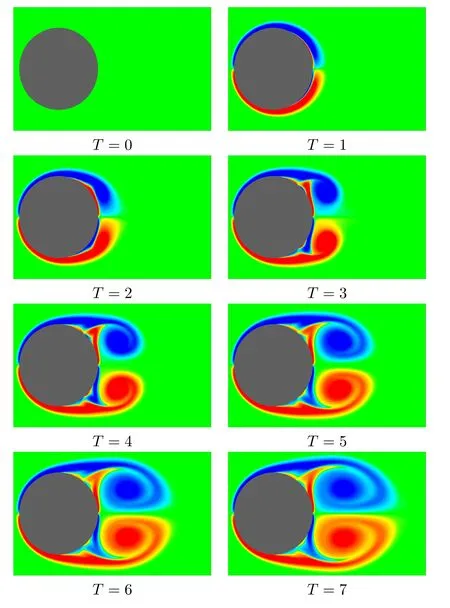
Figure 7:Vorticity of a flow past a circular cylinder at Re=1000 simulated on a grid with 4096×8192 mesh points in the computational domain Ω = (−10,10)2 at different times T ∈[0,7]

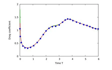
Figure 8:Evolution of the drag coefficient of a circular cylinder at Re = 3000.Red solid line:numerical results on a 4096 × 8192 grid in Ω = (−10,10)2;Green solid line:numerical results on a 8192 × 16384 grid in Ω = (−10,10)2;Blue dots:results from[Koumoutsakos and Leonard(1995)]

As previously mentioned,the flow remains symmetric at the beginning of the simulations for these flows around an impulsively started cylinder.By carrying the time integration over a much longer time intervalT ∈[0,200] instabilities due to round-off errors and to the nonlinearity of the system develop so that the flow becomes non symmetric forT ≥100 at Re = 1000 andT ≥50 at Re = 3000 as it can be seen on Figs.10 and 11 representing the time history of the drag coefficient.After a transient period,an increase of the drag coeffient is observed which stabilizes and oscillates around a mean value.

4.2 Flow around moving bodies

The purpose of this section is to show that the present numerical method is also able to simulate incompressible flows around moving bodies.Let us consider a cylinder which starts to move impulsively att=0 with the sinusoidal translational motion

in a fluid initially at rest for Reynolds number 800.We suppose that the fluid is confined within a rectangular computational domain Ω = [−3;3]×[−1;1] with no-slip boundary condition on∂ΩF.The diameter of the cylinder is equal to 1 and it is initially centered at the origin.The boundary condition(13)at the body surface∂ΩSis enforced through the non exhaustive following right hand side terms which vanish in the case of fixed obstacle:and so on.This terms are respectively taking into account in the convective terms,Laplacian operator and continuity equation.More details can be found in Bouchon et al.[Bouchon,Dubois and James(2012)].

As the obstacle moves from one time step to another,we have to update matrices of the linear systems corresponding to Poisson and momentum equations at each iteration.

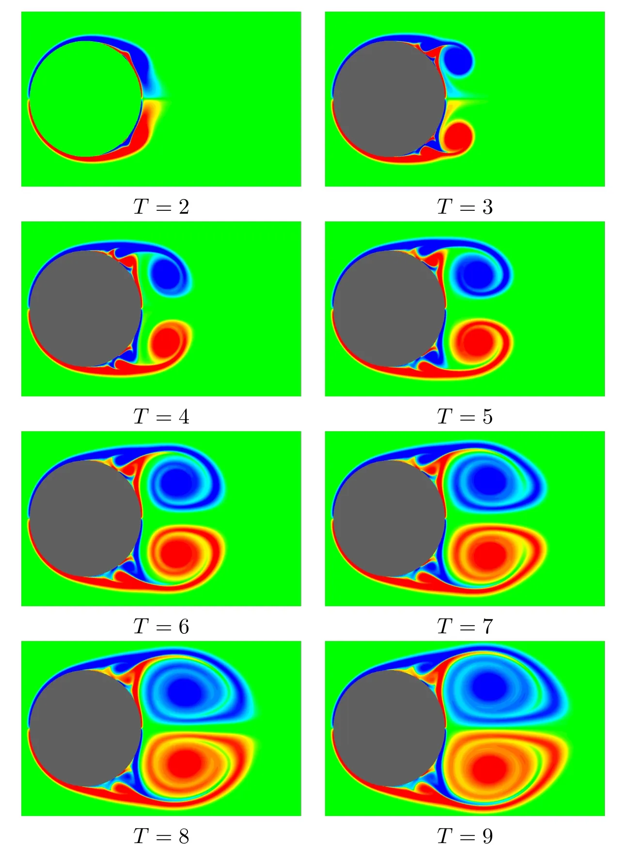
Figure 9:Flow around a circular cylinder at Re = 3000 simulated on a grid with 4096×8192 mesh points in the computational domain Ω=(−10,10)2 at different times T ∈[0,9]

Figure 10:Evolution of the drag coefficient of a circular cylinder for Re=1000 simulated on a grid with 4096×8192 mesh points in the computational domain Ω=(−10,10)2

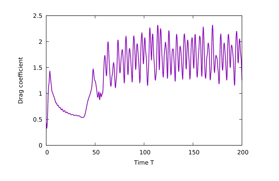
Figure 11:Evolution of the drag coefficient of a circular cylinder for Re=3000 simulated on a grid with 4096×8192 mesh points in the computational domain Ω=(−10,10)2

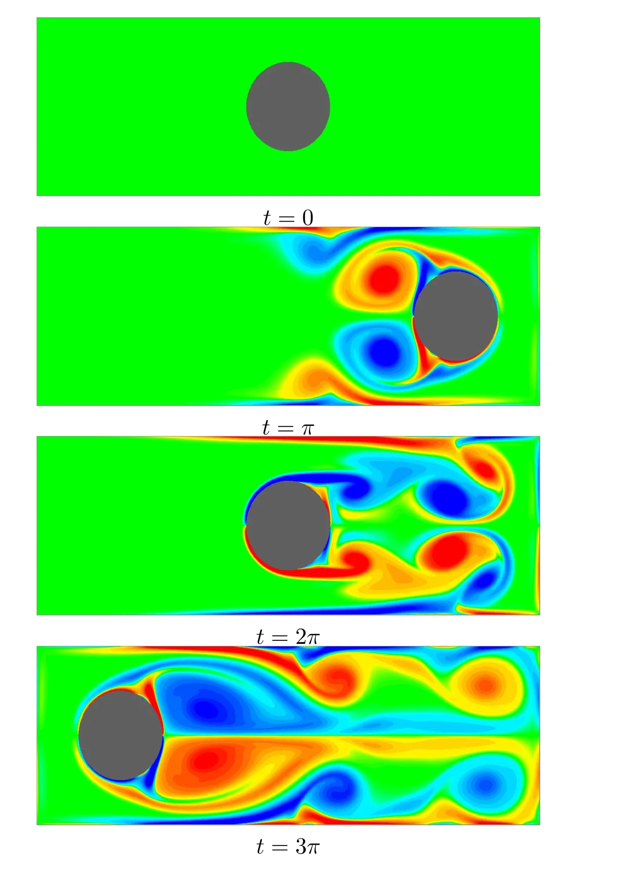
Figure 12:Flow around a moving circular cylinder at Re = 800 in the computational domain Ω=(−3,3)×(−1,1)discretized with 1200×400 mesh points

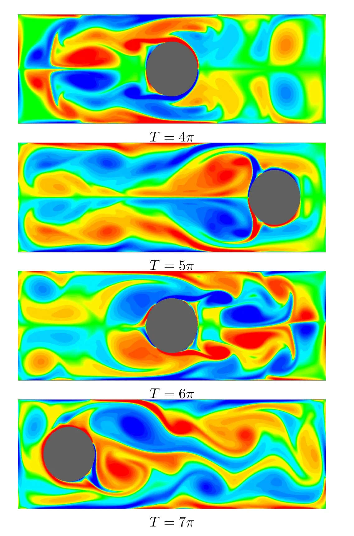
Figure 13:Flow around a moving circular cylinder at Re = 800 in the computational domain Ω=(−3,3)×(−1,1)discretized with 1200×400 mesh points

Therefore,in such configuration,the direct solver requires much more CPU time compared to some iterative solver,which does not require a preprocessing step.For large problems,the faster solver we have found is an algebraic multigrid method(HYPRE BoomerAMG)implemented using the PETSc library[Balay,Abhyankar,Adams et al.(2018b,a)].

A constant mesh sizeh= 5×10−3is used in both directions and the value of the time step,satisfying a CFL stability condition,is 10−3.As shown in Fig.12,vortices interact with each other and also with the boundaries.The flow remains perfectly symmetric untilt= 6π,thereafter the symmetry of the flow is lost due to rounding errors inherent in computer calculations(see Fig.13).

5 Conclusion

We have presented a cut-cell method for the numerical solution of flows past obstacles.We have detailed the numerical method and the computational aspects for fixed obstacles,and shown numerical results for fixed and moving rigid bodies.The parallel version of the algorithm presented here allows computations of flows at Reynolds number up to 3000.The numerical tests confirm some results of the literature,a good agreement is observed with the numerical simulations in Koumoutsakos et al.[Koumoutsakos and Leonard (1995)].We have also shown that the computation of the drag coefficient matches the theoretical square-root singularity predicted by Bar-Lev et al.[Bar-Lev and Yang(1975)].The choice of the size of the box(compared with the grid sizeh)is one of the questions that we would like to investigate with this method in further works,we also would like to deal with rigid bodies following the fluid flow.

Acknowledgement:This research was partially supported by the French Government Laboratory of Excellence initiative noANR-10-LABX-0006,the Région Auvergne and the European Regional Development Fund.The numerical simulations have been performed on a DELL cluster with 32 processors Xeon E2650v2(8 cores),1 To of total memory and an infiniband(FDR 56Gb/s)connecting network.