Multiscale Hybrid-Mixed Finite Element Method for Flow Simulation in Fractured Porous Media

Philippe Devloo,Wenchao Teng and Chen-Song Zhang

1 FEC,Universidade Estadual de Campinas,Brazil.

2 Tracy Energy Technologies,Beijing,China.

3 NCMIS＆LSEC,Academy of Mathematics and System Sciences,CAS,Beijing,China.

Abstract: The multiscale hybrid-mixed (MHM) method is applied to the numerical approximation of two-dimensional matrix fluid flow in porous media with fractures.The two-dimensional fluid flow in the reservoir and the one-dimensional flow in the discrete fractures are approximated using mixed finite elements.The coupling of the two-dimensional matrix flow with the one-dimensional fracture flow is enforced using the pressure of the one-dimensional flow as a Lagrange multiplier to express the conservation of fluid transfer between the fracture flow and the divergence of the one-dimensional fracture flux.A zero-dimensional pressure(point element)is used to express conservation of mass where fractures intersect.The issuing simulation is then reduced using the MHM method leading to accurate results with a very reduced number of global equations.A general system was developed where fracture geometries and conductivities are specified in an input file and meshes are generated using the public domain mesh generator GMsh.Several test cases illustrate the effectiveness of the proposed approach by comparing the multiscale results with direct simulations.

Keywords: Fracture simulation,discrete fracture model,multiscale hybrid finite element,mixed formulation.

1 Introduction

Modeling and simulation of fluid flow in naturally and hydraulically fractured subsurface systems has been a popular research topic in petroleum engineering.According to[Schlumberger(2017)],more than half of the world total oil reserves reside in fractured carbonate reservoirs.Many such reservoirs have their main productivity channel from a network of connected fractures.Oil recovery mechanism in fractured reservoirs,especially shale or tight formations with hydraulically induced fractures,is strongly effected by the accuracy of fracture description.Mathematical models for describing recovery process in complex multiscale fractured formation become more challenging,compared with conventional flow models in homogeneous porous media.In general,there are three types of approaches:(1)continuum models,(2)discrete fracture models,and(3)hybrid models that combine explicit large features and equivalent effective continuum for small features.Naturally each approach has its own advantages and disadvantages.

The Dual Porosity and Dual Permeability(DPDP)model[Barenblatt,Zheltov and Kochina(1960);Warren and Root(1963)]is a well-known continuum model for representing welldeveloped and well-connected small-scale fractures.In this model,besides the rock matrix grid,a structured domain with a set of porosity and permeability is provided to describe the fracture network.The dual porosity models only require small changes to classical reservoir simulators for single media models and can sometimes obtain reasonably good results in practice.To further improve accuracy for simulating oil-water imbibition process,the Multiple INteracting Continua (MINC) model was proposed and applied [Pruess(1985);Wu and Pruess(1988)].Due to the upscaling processes involved in the modeling process,these models will typically fail when fracture length is comparable to the grid size,especially for the scattered fractures[Long,Remer,Wilson et al.(1982)].

Besides continuum representations,another widely studied approach in the reservoir simulation community is the Discrete Fracture Model(DFM),where fractures are modeled as lower dimensional entities [Noorishad and Mehran (1982);Dverstorp and Andersson(1989);Hoteit and Firoozabadi (2005)].The DFMs model the fractures as lower dimensional geometric entities and represent each fracture explicitly with unstructured grids.This approach avoids computing transfer functions between matrix and fracture cells as in continuum models.The DFMs improve accuracy significantly by modeling long fractures.On the other hand,as complexity of the fracture network increases,describing all fractures of different sizes by a finite element or finite volume approximation becomes very expensive.Furthermore,robust and automatic griding algorithms for field-scale simulation of complex fracture networks are still very challenging to construct and it remains an active topic of research;see[Si(2015)]and references therein.To allow independent grids for fracture and matrix domains,many researchers devote efforts to develop and improve the so-called Embedded Discrete Fracture Model(EDFM)or projection-based EDFM that incorporates the effect of each fracture explicitly using non-conforming grids[Lee,Lough and Jensen(2001);Li and Lee(2008);Moinfar,Varavei,Sepehrnoori et al.(2012,2014);Hajibeygi,Al Kobaisi,Bosma et al.(2017)].

Considering the distribution uncertainty and huge quantity of natural fractures in formations,hybrid approaches have been developed to reduce the prohibitive computational cost caused by direct simulation of small-size fractures [Lee,Lough and Jensen (2001)].These approaches simulate fractures of different scales with different models,which combine continuum models and DFM/EDFM.The continuum approach is employed to describe the dense small-scale fractures and DFM/EDFM is used to explicitly model the large-scale fractures[Moinfar,Varavei,Sepehrnoori et al.(2012);Wu,Li,Ding et al.(2014);Jiang and Younis (2016)].Such a methodology has been proved effective by numerical studies;see Moinfar [Moinfar (2013)] and references therein for details.It should be noted that the number of degrees of freedom is still beyond the scope of classical computational methods with homogenizing natural fractures [¸Tene,Al Kobaisi and Hajibeygi(2016)].This motivates the development of an efficient multiscale method for heterogeneous fractured porous media.

The main idea of multiscale Galerkin methods goes back to the work by Babuška et al.[Babuška and Osborn (1983);Babuka,Caloz and Osborn (1994)] and they construct basis functions by solving local flow problems to incorporate fine-scale effects into coarse-scale equations.Thereafter,this idea has been further developed by many researchers and spawned a series of relevant methods,including multiscale finite element method (MsFEM) [Hou and Wu (1997)],multiscale mixed finite element method (MsMFEM) [Chen and Hou (2002);Aarnes (2004)],heterogeneous multiscale method (HMM) [Weinan and Björn (2005)],generalized multiscale finite element method (GMsFEM) [Efendiev,Galvis and Hou (2013)],and multiscale finite-volume method(MsFVM)Jenny,Lee and Tchelepi(2003).During the past few years,multiscale methods have been extended to simulate fluid flow in fractured media.For example,DFM has been integrated into MsFEM by Zhang et al.[Zhang,Huang,Yao et al.(2017)] and GMsFEM by Akkutlu et al.[Akkutlu,Efendiev and Vasilyeva(2016)].

One of the main contributions of this work is the combination of modeling discrete fracture networks with the Multiscale Hybrid-Mixed (MHM) method.The MHM method was originally developed by Valentin,Harder,and Paredes(see Harder et al.[Harder,Paredes and Valentin(2013);Paredes,Valentin and Versieux(2017);Araya,Paredes,Valentin et al.(2013)] for more details) and is a numerical approximation technique geared towards the approximation of conservation laws that incorporate multiple scales.The MHM method has been extended to mixed finite element approximations in Duran et al.[Duran,Devloo,Gomes et al.(2018)],in which the MHM method is described and compared with other multiscale methods such as the Hybrid Discontinuous Galerkin method[Cockburn(2016)]and the Hybrid High-Order method[Di Pietro,Ern and Lemaire(2016)].The extension of the MHM method to the numerical simulation of discrete fracture networks is to extend the boundary fluxes over each polygonal domain with fluxes associated with the fracture flow.In this paper,we propose a multiscale hybrid-mixed finite element method for DFM and describe its implementation in the NeoPZ finite element library[Devloo(1997)].

The rest of this paper is organized as follows.The basis of representing fluid flow through the interfaces of the elements using mixed finite elements is a hybridized version of mixed finite element approximations and is presented in Section 2.The fluid flow in the fracture is modeled using a lower dimensional flux is described in Section 3.Finally numerical examples in Section 4 demonstrate the simulation of flow through porous medium where volumetric flow is combined with fluid flow through fractures.

2 A mixed finite element approximation

In this section,we describe a mathematical formulation for approximating discrete fracture models coupled with the porous media flow.We propose a hybridized mixed finite element formulation,which substantially decreases the size of the discrete linear system.In this formulation,we use a hierarchal grid of two length scales:(1)a coarse-scale structured or unstructured grid based on which global degrees of unknowns are defined,and(2)a finescale unstructured grid is employed to describe long fractures.We note that such a method can also be combined with continuum models in order to take short and medium fractures into account.

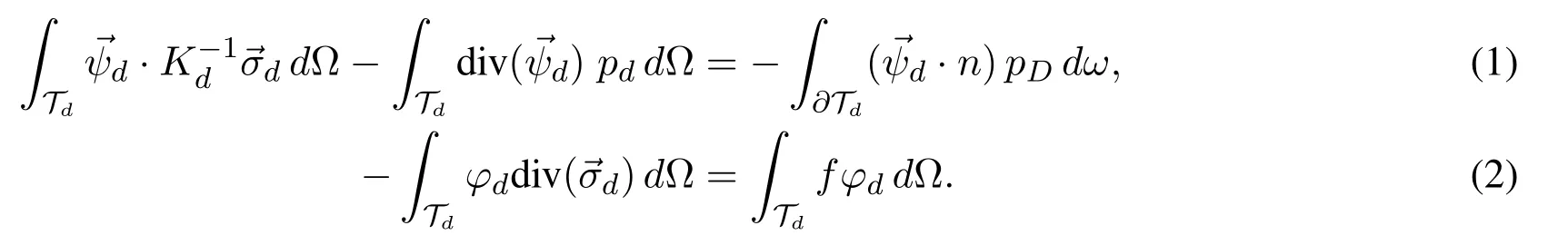
LetTd ⊂Rdbe a polygonal computational domain.The mixed approximation of the Laplace equation onTdcan be formulated as :Finds uch that

2.1 Hybridized mixed finite element approximations

Mixed finite element approximations have the distinct feature that the numerical results of the hybridized formulation are identical to the original formulation.Moreover,when statically condensing the internal fluxes and pressures onto the pressure on the interfaces,the issuing global matrix is symmetric positive definite(SPD).

For simplicity,we restrict our discussion in two-dimensional(d= 2)matrix domain with one-dimensional fractures in this paper.We denote the partition of macro elements asT2:={T2:T2⊂Ω}and the interfaces between macro elements asT1in this case.A hybrid mixed finite element approximation of a flow through porous medium is described as:Find(2,p1)∈Hdiv(T2)×L2(T2)×H1/2(T1)such that

for any(1)∈Hdiv(T2)×L2(T2)×H1/2(T1).

The meaning ofandp1is illustrated graphically in Fig.1:the pressurep1acts as a Lagrange multiplier to enforce the continuity of.Eq.(3) represents the Darcy’s constitutive law of the fluid flow in porous media.The third term corresponds to the pressure at the interfaces of the macro fluxes that acts as a(weak)Dirichlet condition for the macro domain.Eq.(4) represents the two dimensional conservation law.Eq.(5)establishes that the sum of all normal fluxes at the interface between macro elements has to be weakly zero.Furthermore,theHdiv(Td)approximations can be hybridized one side at a time.

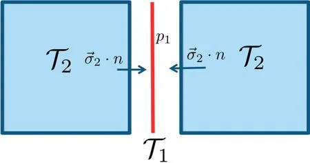
Figure 1:Hybridizing an interface between two H(div)-elements

2.2 The multiscale hybrid-mixed method

The multiscale hybrid mixed (MHM) method is a technique developed towards the numerical approximation of partial differential equations whose solution exhibit multiscale features.Within the MHM framework the normal component of the flux over the macro elements is approximated by piecewise continuous functions.The extension of these flux functions in the interior of the macro domains constitute the MHM basis functions.

To illustrate the concept of the extension of boundary fluxes in conjunction with discrete fracture networks,a square macro domain is used with a fracture as illustrated in Fig.2.The permeability of the matrix is unitary and the permeability of the fracture times fracture width is 100.

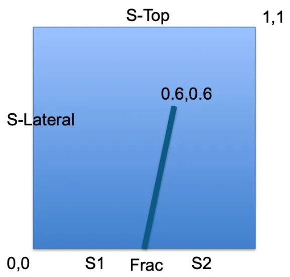
Figure 2:A representative MHM domain with fracture

•Fig.3 shows the pressure extension functions associated with constant fluxes associated with front and back sides of the domain.The impact of the embedded fracture is easily noted.The tip of the fracture,where the fluid convected by the fracture is injected in the domain,generates a singularity.

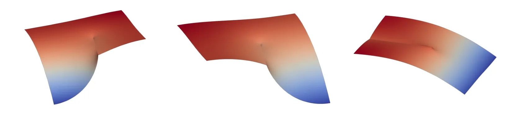
Figure 3:Pressure extension associated with constant fluxes injected in S1,S2,and S-Top

•Fig.4 shows the pressure for a lateral flux and for a unitary flux injected at the point of the fracture.This is an innovation contributed by this work.The piecewise polynomial fluxes associated with the sides of the macro domain are augmented with a point flux at the intersection of the fracture with the boundary of the MHM macro domain.

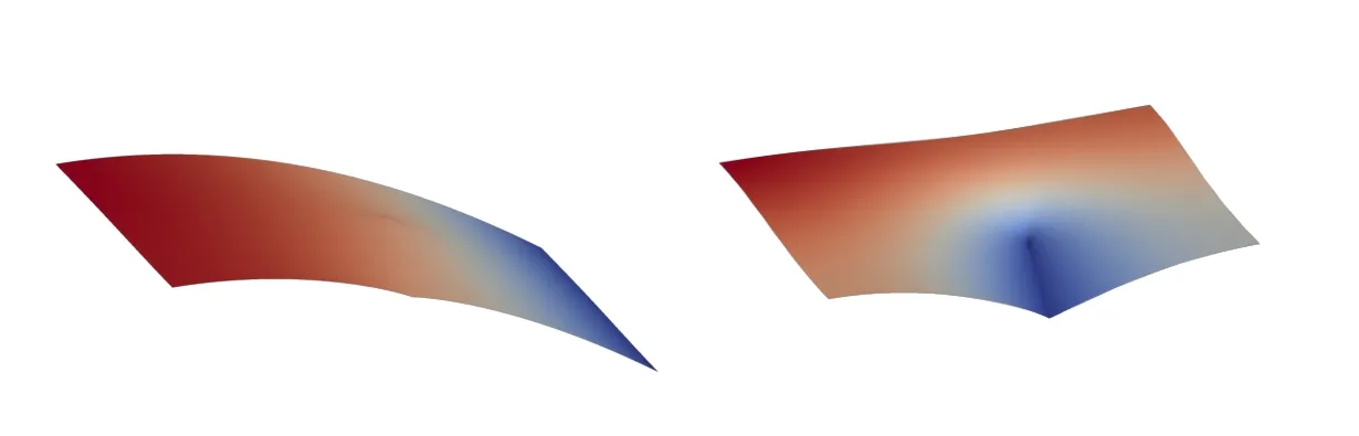
Figure 4:Pressure extension associated with constant fluxes injected in S-Lateral and Frac

Observing the function extensions for this domain with one fracture,the capability of the MHM method for simulating multiscale problems is apparent-the singularity caused by the fracture point is isolated in the interior of the domain.The fine mesh used to capture the details of the flow pattern is confined in the interior of the domain.The size of global system of equations is determined uniquely by the number of boundary fluxes and is,therefore,not affected by the resolution of the interior mesh.

2.3 MHM and H(div)approximations

In MHM approximations the computational domain is discretized in two levels:a coarse polygonal mesh which is referred to asmacro domainsand a fine discretization on micro elements meshing the interior of each macro domain.This two-level discretization is illustrated in Fig.5.The macroscopic fluxes between the macro elements represent the coarse-grained response of the fluid flow problem.The approximations using fine meshes at the interior of each macro element capture the detailed behaviour of the fluid flow.

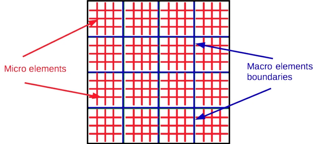
Figure 5:Macro and micro elements for partitioning of Ω

When applying the MHM method usingH(div) approximations at the interior of each macro domain [Duran,Devloo,Gomes et al.(2018)],the MHM method amounts to applying shape function restraints of the fine scale approximations to the space of the macro fluxes(see[Díaz Calle,Devloo and Gomes(2015)]for example).As such the formulation of the MHM method is identical to the mixed finite element formulation.The difference is that in MHM the flux approximation space is partitioned between macro fluxes associated with the boundary of the macro domaines and internal fluxes and pressures associated with the interior.

3 Coupling fractures with surrounding porous media

Our work is based on the DFM formulation,which represents fractures as simplified(n−1)-dimensional entities in ann-dimensional domain.As a result,fractures distributed in 2D space will be discretized in 1D form.Fig.6 shows a porous rock with one fracture to illustrate the idea of DFM.The matrix domain is represented by Ωm,and the fracture domain by Ωf.The assumption of DFM is that all variables remain constant in the cross direction of the fractures.Therefore,the only difference between the single-porosity model and DFM is the integral computation for the fracture domain.In DFM,the fracture aperture can be taken as a factor in front of the 1D integral to simplify the problem considerably.

3.1 Modeling fluid flow in a discrete fracture network

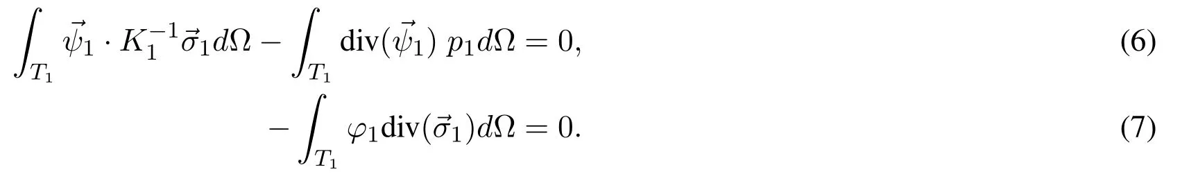
The fluid flow in the fractures is modeled using a mixed approximation.This formulation is based on previous work of the authors published in[Castro,Devloo,Farias et al.(2016)].The fluid flow in a single fracture can be modeled as:Find(1)∈Hdiv(T1)×L2(T1)such that

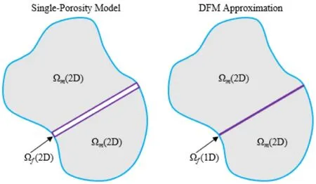
Figure 6:Schematic representation of DFM (modified from Karimi-Fard et al.[Karimi-Fard and Firoozabadi (2001)])

When fractures intersect,the conservation of mass states that the sum of the normal fluxes at the intersection should sum to zero.The conservation at the intersection is imposed by the introduction of a Lagrange multiplier which has the physical quantity of the pressure at the intersection.The statement then becomes:Find(1,p0)∈Hdiv(T1)×L2(T1)×L2(T0)such that

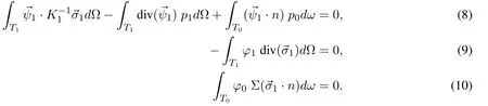
Eq.(8) expresses the constitutive law of one-dimensional fluid flow in the fracture.p0represents the pressure at the fracture intersections.Eq.(10)expresses the conservation of mass at the fracture intersection.The flow in intersecting fractures is illustrated in Fig.7:the red squares illustrate intersection points where 2,3,or 4 fractures meet.

3.2 Coupling flow in porous media and discrete fracture network

If there is fluid exchange between the two dimensional fluid flow and the fracture,the conservation of mass requires that the fluid flow that leaves the two dimensional domain enters as a source term for the one dimensional conservation law.Reciprocally,the pressure of the fluid in the fracture acts as a pressure boundary condition for the two dimensional matrix fluid flow.The simulation spaces that will interact are listed as follows:

Figure 7:Illustration of 1D fluxes in a two dimensional domain

•two dimensional fluxesand weight functions

•two dimensional pressuresp2and weight functionsϕ2,

•one dimensional pressuresp1and weight,functionsϕ1,

•one dimensional fluxesand weight functions

•zero dimensional pressuresp0and corresponding weight functionsϕ0.

In turn,we can now write down the issuing variational statement as

Each equation in the above system corresponds to either a physical conservation law or a constitutive relation:

1.The first equation implements the constitutive law in two dimension indicating that the pressures in the fractures act as pressure boundary conditions.

2.The second equation represents the mass conservation in two dimension.

3.The third equation implements the constitutive law in the fractures where the pressures at the end of the fractures (zero dimensional pressures) act as pressure boundary conditions.

4.The fourth equation implements mass conservation in the fracture where the normal fluxes of the two dimensional elements act as external sources.

5.The fifth equation represents mass conservation at the points where multiple fractures intersect.More than two subdomains can be connected through an interface(hence the generic Σ).This is the case when fluxes along one-dimensional manifolds in the computational domain come together.For example,Fig.7 shows seven line segments linked together by three point-wise pressures.

The system of Eqs.(11)-(15)looks more complicated than it actually is.For simplicity,we may write these equations in the following saddle-point form:

Here we denotetijthej-th term of equationi(index starting from 1) then the correspondence between the integrals and NeoPZ integrals are

• t11,t12,t21,r2are computed by a regular two dimensionalH(div)element;

• t33,t34,t43,r1are computed by a one dimensionalH(div)element;

• t14,t41are computed by a one dimensional interface element which lies between the two dimensionalH(div)element and the one dimensionalH(div)element;

• r3is computed by a one dimensional element associated with a Dirichlet boundary condition;

• t35,t53are computed by an interface element between the one dimensionalH(div)elements and point elements at the intersection of fractures.

It is worthy to observe that static condensation can be applied at different levels to reduce the size of the global system of equations:

•For each micro element,the internal fluxes and all but one pressure equation can be condensed on the boundary fluxes of the element.

•For each macro element,all internal fluxes and all but one pressure equation can be condensed on the boundary fluxes of the macro domain.The flux in the fractures where they intersect with boundaries of the macro domain can not be condensed.

Hence the global system of equations corresponds to the following variables:

•the macro fluxes,

•average pressure of each macro domain,

•zero dimensional fluxes at the intersections of the fractures with the macro domain boundaries(one equation for each intersection).

This means that,after static condensation,we obtain a much smaller global linear system to solve;see the numerical comparison in the next section.Comparing to the MHM approximations without fracture flow,the global system of equations is incremented by one equation for each intersecting fracture.

4 Numerical experiments

In this section,we perform a few preliminary numerical experiments in order to validate the proposed numerical method,which shall be denoted as MHDFM for convenience.Simulations are run on a personal computer.For comparison,we use a commercial software to obtain DFM and full-resolution direct simulation results.We always set the permeabilities of fractures and surrounding porous medium to beK1=Kf= 105andK2=Kp=1,respectively.

The proposed algorithm is implemented using the object oriented framework for development of finite element algorithms NeoPZ.The NeoPZ environment implements one,two and three dimensional hp-adaptive finite element approximations.Modules are dedicated to the geometric approximation,the definition of the approximation space and the definition of the differential equation to be approximated.In this work we combine one and two dimensionalH(div)approximation spaces through the use of interface elements.

4.1 Orthogonal fractures

A homogeneous 2D problem with two orthogonal fractures is considered (see Fig.8(a)),where a“+”-shaped fracture network located at the center of the quadratic domain.No-flow boundary conditions are applied at the top and bottom,while the pressure values are set top= 1 andp= 0 at the left and right boundaries.According to the length scales specified in Fig.8(a),the fractures with aperturea=0.04 are fully resolved using at least 225×225 grid cells (fully resolved direct simulation).For the DFM method,an unstructured grid is employed;see Fig.8(b).For the MHDFM method,a 13×13 coarse grid is used;see Fig.8(c).

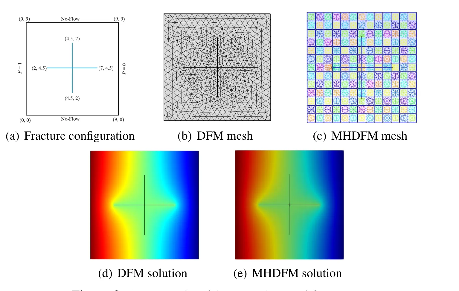
Figure 8:An example with two orthogonal fractures

Figs.8(d) and 8(e) illustrate the solutions from the DFM and MHDFM approaches,respectively.The colors in our simulation result look different than the DFM result because we cannot match the color mapping used in the commercial software exactly.But the numerical values are very close to each other.In order to make a quantitative comparison,we give Fig.9 that represents the pressure along the horizontal center line of the domain.The seemingly horizontal line segment with little pressure loss in the plot matches with the fracture domain from(2,4.5)to(7,4.5)due to the fracture permeability is very large compared with the matrix permeability.The pressure obtained by MHDFM shows excellent agreement with DFM and direct simulation results.Note that the role of the vertical fracture is less important than that of the horizontal line one.The results from MHDFM,DFM,and direct simulation are close;see Tab.1.Compared to the fully resolved fine-scale solution and conventional DFM result,the total flow rate computed by MHDFM is almost identical with a discrepancy less than 2.56×10−3.

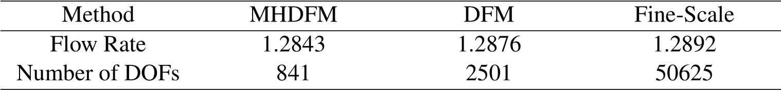
Table 1:Computational flow rate comparison

4.2 Rotated orthogonal fractures

This example also contains two orthogonal fractures,which are located at (2,7;7,2) and(7,7;2,2) respectively.The numerical total flow rates computed by DFM and MHDFM are 1.6122 and 1.6081,respectively.The relative difference is 2.54×10−3.

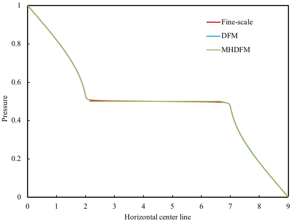
Figure 9:Comparison of pressure on the horizontal center line(y =4.5)

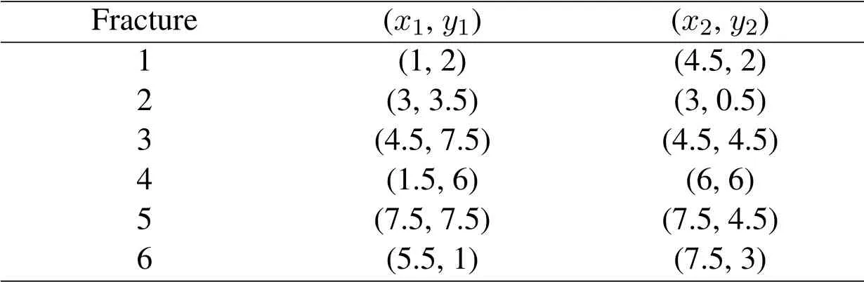
Table 2:Fracture(end-points)distribution

4.3 Nonorthogonal fractures

Another homogeneous 2D case with two nonorthogonal intersecting fractures(see Fig.11)is also tested.The boundary condition and other parameters are the same as in the first case and the only difference is the fracture distribution.The two fractures are respectively located at(3,8;6,2)and(5,7;2,3).The total flow rates computed by DFM and MHDFM are 1.2724 and 1.2661,respectively.The relative difference is 4.95×10−3.

4.4 Disjoint fracture networks

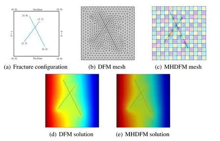
Figure 11:A DFM example with two nonorthogonal fractures

We summarize the size of global linear systems in different methods in Tab.3.Except the first example,it is difficult for us to obtain computational meshes for the direct simulation method in order to resolve the fracture fully.We can see that we are able to reduce the size of global systems to solve by using the proposed multiscale hybrid-mixed method.Moreover,we make a few comments on the method:

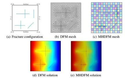
Figure 12:A more complicated example of fracture network

•In MHDFM,we useH(div)approximation for the flux and pressure variables.This requires more degree of freedom on each element,but gives better accuracy;

•For convenience and load balance,we use uniform finer meshes in the MHDFM simulation.This can be replaced by locally refined meshes to reduce computational cost;

•In this section,we focus on validation of the method and did not pay attention to the actual computational efficiency or parallelization of MHDFM.These aspects are the potential advantages of MHDFM and deserve further studies in the future.

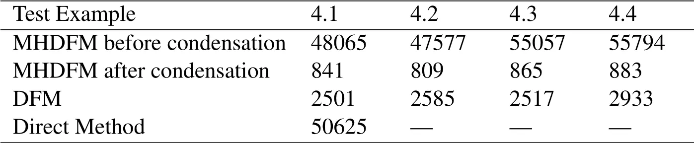
Table 3:Numbers of degrees of freedom for MHDFM,DFM,and direct method

5 Conclusions

In this paper,a discrete fracture model is approximated using mixed finite elements.The fluid flow in the fracture is modeled using lower dimensional elements applied to a Laplace-Beltrami operator.Fracture intersections are modeled using a Lagrange multiplier enforcing local conservation.The pressure in the fracture acts as a boundary condition for the two dimensional flow.The Multiscale Hybrid Method is applied to separate the local features of the fracture-reservoir coupling from the global features of fluid flow.The resulting numerical model leads to a very reduced global system of equations.In turn we are able to reduce computational cost to an acceptable level.Results of the proposed numerical model are compared with the standard DFM simulation and the finescale simulations using finite volume techniques.In all cases the difference in flow rate are less than 1%.

6 Acknowledgements

Zhang was partially supported by the National Key Research and Development Program of China(Grant No.2016YFB0201304)and the Key Research Program of Frontier Sciences of CAS.Devloo acknowledges the financial support from CNPq-the Brazilian Research Council (Grant No.305823/2017-5).This work is carried out during Devloo’s visit to Beijing Institute of Scientific and Engineering Computation(BISEC),China.