A Simple FEM for Solving Two-Dimensional Diffusion Equation with Nonlinear Interface Jump Conditions

Liqun Wang,Songming Hou and Liwei Shi

1 China University of Petroleum-Beijing,Deptartment of Mathematics,College of Science,Beijing,102249,China.

2 Louisiana Tech University,Deptartment of Mathematics and Statistics,LA,Rustion,71272,USA.

3 China University of Political Science and Law,Deptartment of Science and Technology,Beijing,102249,China.

Abstract: In this paper,we propose a numerical method for solving parabolic interface problems with nonhomogeneous flux jump condition and nonlinear jump condition.The main idea is to use traditional finite element method on semi-Cartesian mesh coupled with Newton’s method to handle nonlinearity.It is easy to implement even though variable coefficients are used in the jump condition instead of constant in previous work for elliptic interface problem.Numerical experiments show that our method is about second order accurate in the L∞norm.

Keywords:Finite element method,parabolic equation,interface problems,nonlinear jump conditions.

1 Introduction

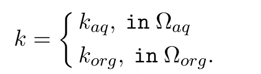
Parabolic problems with nonhomogeneous flux jump condition and nonlinear jump condition are often encountered in scientific computing and engineering.For example,in Radu et al.[Radu,Meir and Bakker (2004);Hetzer and Meir (2007);Bakker and Meir (2003)],a numerical model is introduced to describe the concentrationuof an ionIin aqueous solution Ωaqand adjoining polymeric membrane Ωorg.Since the diffusion coefficients of the aqueous solution and of the membrane are different,this an interface problem with interface Γ at the membrane.The equations for the problem are as follows:

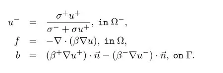
The ion flux continuity across the interface gives a flux jump condition

The analyte ionIexchanges with ionJof the same valency at the interface,therefore

which can be rewritten as the nonlinear jump condition

Given proper boundary condition and initial condition,the above mentioned problem is a one-dimensional nonlinear interface problem with homogeneous flux jump condition.The numerical solution of interface problems has attracted much attention in recent years.The numerical method using non-body-fitted grids for elliptic interface problem was first proposed by Peskin[Peskin(1977)].After that,various numerical methods are developed,including the immersed interface method(IIM)[LeVeque and Li(1994);Li and Ito(2006);Li (1998)],the immersed finite element method(IFEM) [Li,Lin and Wu (2003);He,Lin and Lin(2011);Gong,Li and Li(2008)]and its partially penalized version[Lin,Lin and Zhang (2015)],the immersed finite volume element method(IFVE) [Ewing,Li,Lin et al.(1999)],the matched interface and boundary method(MIB)[Xia,Zhan and Wei(2011);Yu,Zhou and Wei (2007);Zhou,Zhao,Feig et al.(2006)],the non-traditional finite element method(NTFEM)[Hou,Wang and Wang(2010);Hou,Song,Wang et al.(2013);Hou,Li,Wang et al.(2012)],the weak Galerkin method[Mu,Wang,Wei et al.(2013)],the kernelfree boundary integral(KFBI)method[Ying and Henriquez(2007)],and so on.Gradient recovery technique[Guo and Yang(2018,2017)]is applied to improve the accuracy of the gradient.

In this paper,we propose a numerical method for a much extended scope of problems,which are two-dimensional parabolic interface problems with nonhomogeneous flux jump condition and nonlinear jump condition.Motivated by the numerical model described by Eqs.(1)-(3),and inspired by the traditional finite element method(TFEM) for solving elliptic interface problem we proposed in Wang et al.[Wang and Shi(2014)],we propose a new numerical method for solving the two-dimensional parabolic interface problem with nonhomogeneous flux jump condition and nonlinear jump condition.We use traditional finite element method coupled with Newton’s method to deal with these two special kinds of jump conditions and use Crank-Nicolson scheme to deal with the time derivative.The reason we did not use the NTFEM is because the nonlinear term of this problem is special.It comes from the jump condition.Normally it is effective to use Newton’s method to linearize the nonlinear system.However,when the nonlinearity comes from the jump condition along the interface,we need to solve the nonlinear system at the local cell for a time step if we use the NTFEM,and the result of this system will be a linear combination of the unknown solution located at the vertices of the element cell.Newton’s method need to have an initial entry at every iteration step.However,the NTFEM can only provide an unknown linear combination,which will cause a serious problem at the linearization part.That is why we choose to use the TFEM.Compared with our recent work on elliptic interface problem with nonlinear jump condition in[Wang,Hou and Shi(2017)],the new contributions include:first,for the parabolic interface problem we need to use Crank-Nicolson’s method to handle the time derivative term.This needs to be done carefully with presence of interface.Second,in our previous work,the coefficientsσ,σ+andσ−are all constants for simplicity.In this paper,all these are assumed to be variables depending on both time and space,which makes the nonlinear scheme more difficult to derive.Numerical examples show that our method is very effective and stable,it is efficient for matrix coefficient and sharp-edged interface,and can achieve about second order accuracy in theL∞norm.

2 Mathematical formulation

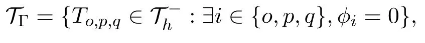
In this paper,we consider a parabolic interface problem defined on an open bounded domain Ω⊂R2cross with a time interval [0,T].Let Γ be an interface that dividesΩ into disjoint open subdomains,Ω−and Ω+,henceAssume that the boundary∂Ω and the boundary of each subdomain∂Ω±are Lipschitz continuous as submanifolds.Since∂Ω±are Lipschitz continuous,so is Γ.Therefore a unit normal vector of Γ can be defined a.e.on Γ,see Fig.1.

Figure 1:Setup of the problem

We seek solutions of the variable coefficient parabolic problem away from the interface Γ given by

in which= (x,y) denotes the spatial variables andis the gradient operator.The coefficientis assumed to be a 2×2 matrix that is uniformly elliptic on each disjoint subdomain,Ω−and Ω+,and its components are continuously differentiable on each disjoint subdomain,but they may be discontinuous across the interface Γ.The righthand sidef()is assumed to lie inL2(Ω).Note thatfis piecewise defined on two sides of the interface.

The flux jump condition along the interface Γ is given by

and the nonlinear jump condition along the interface Γ is prescribed by

The”±”superscripts refer to limits taken from within the subdomains Ω±.

Finally,we prescribe initial and boundary conditions

for a given functiongon the boundary∂Ω andu0on the domain Ω.

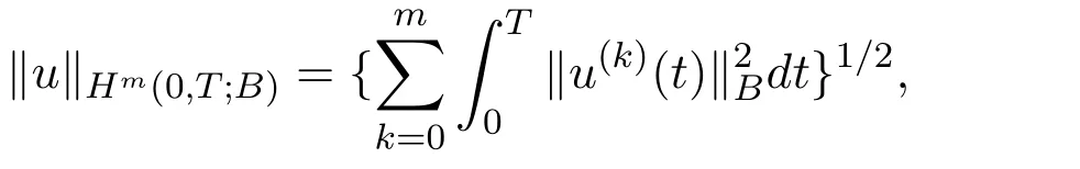
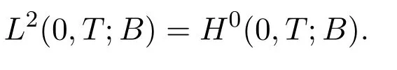
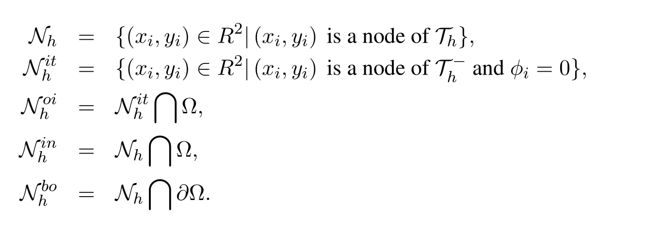
In order to derive the weak formulations of the mathematical model defined by Eqs.(4)-(7),we need to define some notations as in Chen et al.[Chen and Zou(1998);Huang and Zou(2002)].For a Banach spaceB,define

whereis the norm ofHm(0,T;B)and is given by

and

Now we are ready to derive the weak formulation of Eq.(4).Using the traditional finite element method,with the standard procedure of multiplying by a test functionψand integrating by parts,we deduce the weak solution:

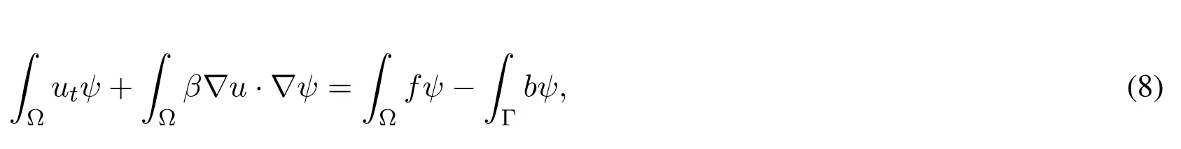
whereψis inH10(Ω).

Below the weak formulation is employed to solve the parabolic interface problem.First divide the time interval [0,T] intontequally spaced subintervals [tn−1,tn],n=1,2,··· ,nt,withtn=n∆t,∆t=T/nt.According to the Crank-Nicolson method in Wang et al.[Wang and Shi (2015)],the following semidiscrete problem of Eq.(4) is derived:

Further,the weak formulation of the semidiscrete problem reads

3 Numerical method

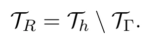
In this section,a numerical method is implemented to solve the nonlinear system described in Eqs.(4)-(7).The grid used in this paper is the semi-Cartesian grid introduced in Wang et al.[Wang and Shi(2014);Wang,Hou and Shi(2017);Xie,Li and Qiao(2011);Wang,Li and Lubkin(2014)],see Fig.2.Letφ(x,y)be a level set function.For simplicity,we useφito representφ(xi,yi)in the following discussion,wherexi,yiis a grid point.

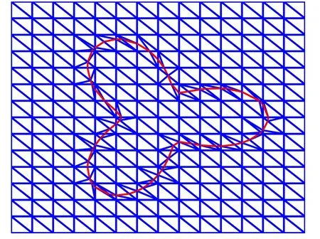
Figure 2:A schematic illustration of semi-Cartesian triangulation

For any cellTo,p,q,o,p,q ∈{1,2,··· ,N},whereNis the number of grid points,we define two sets bellow:

Then the body-fitting triangulationThof the domain Ω is obtained asThe setTΓof interface cells is defined by

and Γhis used to define the interface segment on the interface cellT.The setTRof regular cells is defined by

Note that for body-fitted grid the interface does not cut through the triangle,it only touches one vertex or one side of the triangle.Therefore there are only two kinds of interface cells,see Fig.3.It is this desirable property that ensures our method straightforward to implement.

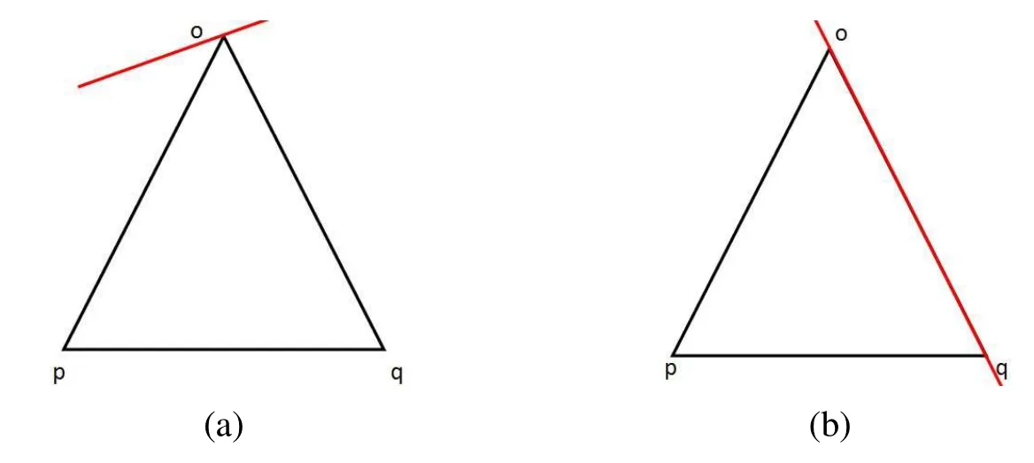
Figure 3:Interface cells

Now we introduce the canonical piecewise linear finite element spaceXhon the triangulationTh:

whereP1(τ)denotes the space of linear functions onτ.

We shall construct an approximate solution to the interface problem by using the spaceXh,but taking into account the jump conditions.First note that the flux jump condition[(β∇u)· n] =balong the interface Γ is already absorbed into the weak formulation.Hence,the most important and challenging part is the nonlinear jump condition prescribed in Eq.(6).The approximate solution is piecewise linear on both subdomains Ω−and Ω+,but discontinuous along the interface Γ.

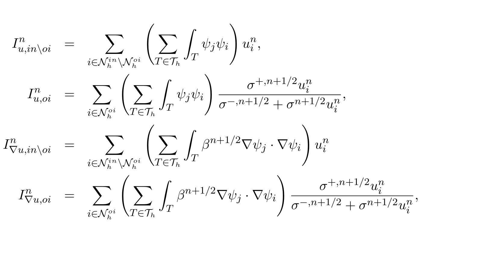
For grid points that are involved in two different solutions,like pointoin Fig.3(a)or pointso,qin Fig.3(b),we have the following definitions:for any cellthen

and ifT ∈T −h,then

Next we have notations defined as below [He,Lin and Lin (2011);Wang,Hou and Shi(2017)]:

Also,i ∈Nis used to denote(xi,yi)∈N.

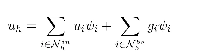
With these notations,a globally piecewise linear approximationuhcan be defined as

Before deriving the discrete formulation for the weak Eq.(10),for simplicity consideration,let

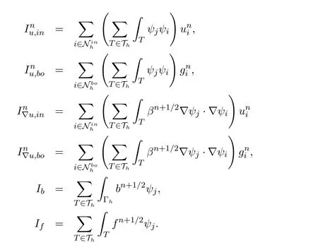
Then we have the following method:

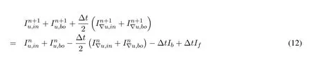
Method 3.1.Find a solution uh such that for all ψj ∈Xh,we have

Although we can get this discrete Eq.(12),it is a nonlinear equation.In this paper,we use the Newton’s method to linearize and solve the problem.Unlike other nonlinear problems having a nonlinear term with specific definition in the governing equation defined on the whole domain,the nonlinear part of this problem comes from a local place:it located at the interface.Therefore we need to separate the interface points from the interior points.Then the nonlinear term needs to be coupled in the governing equation such that we can use Newton’s method to linearize the system.Sinceσis nonzero in this paper,the solution jump is nonhomogeneous,that means there will be two solutionsu±and two governing equations defined on the point located at the interface.When we are calculating the Jacobian matrix of the nonlinear system,we need to figure out it is with respect to which equations and which unknowns.This is a tricky issue for the linearization procedure.

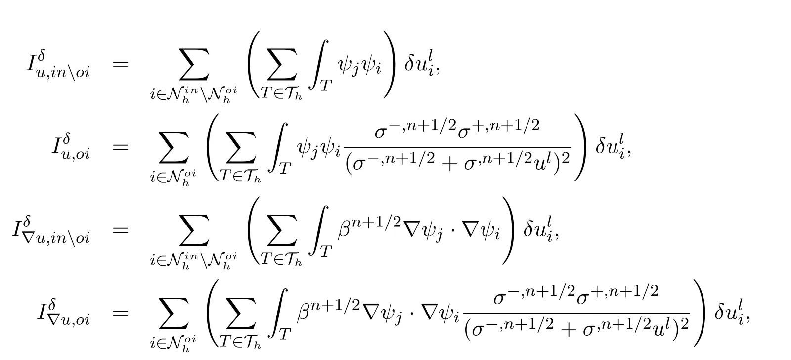
Based on the above discussion,and take the nonlinear jump condition into consideration,define

then we have the following residual equation:

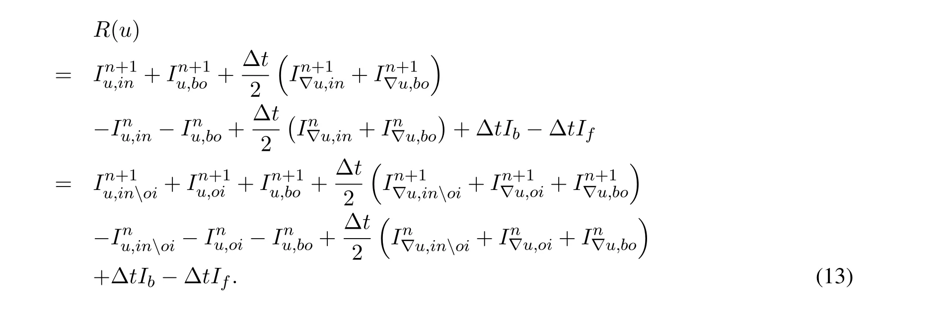
Hence the iteration method can be written as

wherelrefers to the iteration step of the Newton’s method,ulis the unknown vector,such thatis the Jacobian matrix.Let

with the notations defined above,and from Eqs.(13) and (14),we have the following method:

Method 3.2.Find a solution uh such that for all ψj ∈Xh,we have

Remark 3.1.In our implementation,the integrals are computed with Gaussian quadrature rules.For each triangular cell,the midpoint of each edge is denoted by pij.In numerical computation,the average of three f(pij)in each cell is utilized.

4 Numerical experiments

In this section,we use three specific examples to testify the efficiency of our method(Method 3.2)for solving the two-dimensional diffusion equations with nonlinear interface jump conditions.

In all numerical experiments below,the level-set functionφ,the coefficientsβ±,σ±,σ,and the solutionu+in Ω+are given.Hence

Since the solutions are given,gandu0are obtained as a proper Dirichlet boundary condition and an initial condition.The right hand side functions of the PDEs are evaluated using the left hand side and the true solution.

All the examples are defined on the domain[−1,1]×[−1,1]×(0,1].

The termination condition for the Newton iteration method in this paper is

All errors in solutions are measured in theL∞norm in the whole domain Ω.

Example 1.The level-set function φ,the coefficients β±,σ±,σ and the solution u+aregiven as:

In this example,the coefficients β± are diagonal matrices,σ± and σ are variable coefficients depending on the space.Fig.4(a) and Fig.4(b) show respectively the numerical solution and the error at T=1with our method using a20×20×10grid.Fig.4(c) shows the geometry of the level set function and a semi-Cartesian grid with 20 grid points in both x and y directions.Tab.1 gives the errors on different grids.Numerically,the method is second order accurate and the Newton’s iteration steps remain less than7,which demonstrates the stability of our method.

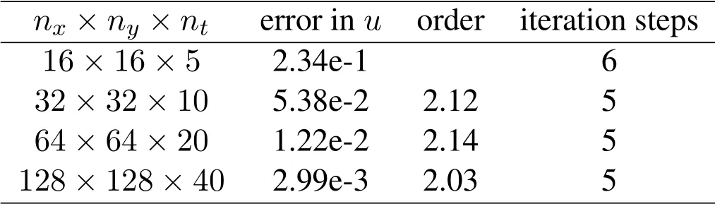
Table 1:Numerical results for Example 1

In the next two examples,the coefficientsβ±are symmetric matrices,σ±andσare variable coefficients depending on space and time.

Example 2.The level-set function φ,the coefficients β±,σ±,σ and the solution u+are

Figure 4:Numerical results for Example 1

Fig.5(a) and Fig.5(b) show respectively the numerical solution and the error at T= 1with our method using a20×20×10grid.Fig.5(c)shows the geometry of the level set function and a semi-Cartesian grid with 20 grid points in both x and y directions.Tab.2 gives the errors on different grids.Numerically,the method is second order accurate and the Newton’s iteration steps is3.

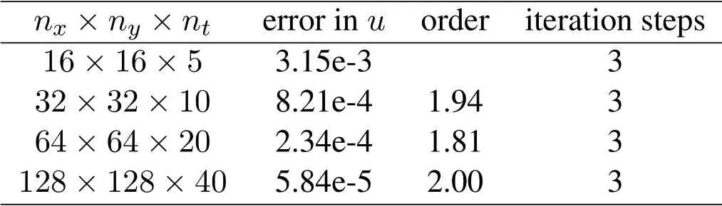
Table 2:Numerical results for Example 2

Example 3.The level-set function φ,the coefficients β±,σ±,σ and the solution u+are given as:

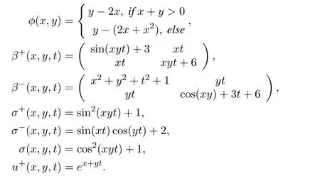
Fig.6(a) and Fig.6(b) show respectively the numerical solution and the error at T= 1with our method using a20×20×10grid.The geometry of the level set function and a semi-Cartesian grid with 20 grid points in both x and y directions are shown in Fig.6(c).Tab.3 gives the errors on different grids.Numerically,the method is second order accurate and the Newton’s iteration steps remain less than6.

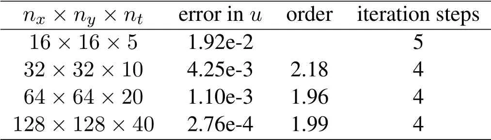
Table 3:Numerical results for Example 3

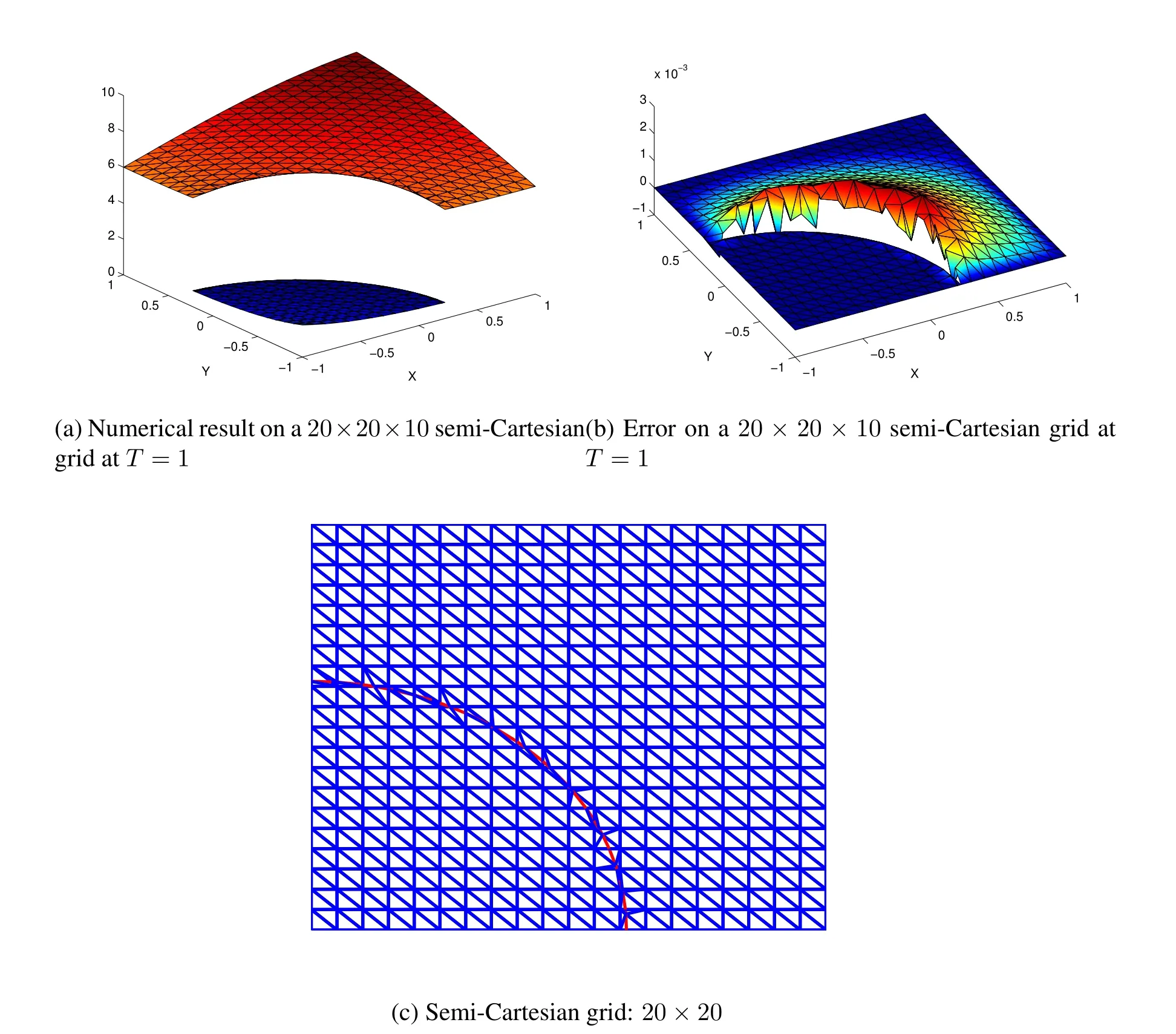
Figure 5:Numerical results for Example 2

5 Conclusion

Figure 6:Numerical results for Example 3

We developed a simple,efficient numerical method for matrix-valued coefficient parabolic equations coupled with nonhomogeneous flux jump condition and nonlinear jump condition.We used TFEM coupled with Newton’s method to deal with these two special and complicated jump conditions and used Crank-Nicolson’s scheme for time derivative.The coefficients in the jump conditions are variable instead of constant in our previous work.We found that our previous work on NTFEM is not suitable treating such problem due to the linearization part,and this is not a trivial extension of our previous work on TFEM for elliptic interface problem due to the time derivative and the coefficients not being constant in the jump conditions.This is not a trivial extension of the previous work on the one dimensional nonlinear interface problem either,because the geometry in two dimensions is much more complicated than one dimension.As far as we know,a solver for this problem has not been reported in the literature.Extensive numerical experiments indicate that the method is about second-order accurate in theL∞-norm,and it is stable even for problems with very complicated interfaces.

Acknowledgement:L.Shi’s research is supported by National Natural Science Foundation of China(No.11701569).S.Hou’s research is supported by Dr.Walter Koss Professorship made available through Louisiana Board of Regents.L.Wang’s research is supported by Science Foundations of China University of Petroleum-Beijing(No.2462015BJB05).