An Augmented IB Method＆Analysis for Elliptic BVP on Irregular Domains

Zhilin Li,Baiying Dong,Fenghua Tong and Weilong Wang

1 CRSC＆Department of Mathematics,North Carolina State University,Raleigh,NC 27695-8205,USA.

2 School of Mathematics and Statistics,Ningxia University,Yinchuan,750021,China.

3 College of Mathematics and System Sciences,Xinjiang University,Urumqi,830046,China.

Abstract:The immersed boundary method is well-known,popular,and has had vast areas of applications due to its simplicity and robustness even though it is only first order accurate near the interface.In this paper,an immersed boundary-augmented method has been developed for linear elliptic boundary value problems on arbitrary domains (exterior or interior) with a Dirichlet boundary condition.The new method inherits the simplicity,robustness,and first order convergence of the IB method but also provides asymptotic first order convergence of partial derivatives.Numerical examples are provided to confirm the analysis.

Keywords: Immersed boundary method,augmented approach,convergence,derivative computing.

1 Introduction

In this paper,we develop an augmented immersed boundary method for linear elliptic boundary value problems (BVP) on arbitrary domains.Since its introduction in 1970’s,the Immersed Boundary (IB) method [Peskin (1977)] has been flourished in many fields including mathematics,engineering,biology,computational fluid dynamics(CFD),see for example Peskin et al.[Peskin and McQueen (1995)] for reviews and references therein.The IB method is not only a mathematical modeling tool in which complicated boundary conditions can be treated as source distributions but also a numerical method in which a discrete delta function is utilized to spread the singular source to nearby grid points.The IB method is robust,simple,and has been applied to many problems.

The problem of interest in this paper is to solve the following boundary value problem numerically

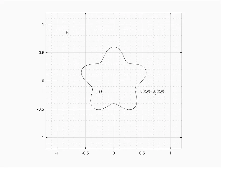
Figure 1:A diagram of an interior boundary value problem on an irregular domain that is embedded in a Rectangular domain with a uniform grid.The geometry is used in numerical experiments in Section 5

For wellposedness requirement of the problem,we also assume thatβ(x)≥β0>0,σ(x)≥0,β(x)∈C(Ω),σ(x)∈C(Ω),andf(x)∈C(Ω),so thatu(x)∈C2(Ω).

It is challenging to solve the problem above both in discretization and solving the resulting linear system of equations after the discretization.Various efforts can be found in the literature including the capacitance matrix method,fictitious domain methods,boundary integral methods if the coefficients are constants,and the augmented immersed interface method[Hunter,Li and Zhao(2002);Li,Zhao and Gao(1999)]etc.,and some immersed boundary(IB)based methods.Most of the methods mentioned are relatively sophisticated.The purpose of this paper is to develop the IB method for the irregular domain problem that has the same nature as the original IB method in terms of the accuracy and the simplicity.The idea is to extend the setting to a rectangular domain so that the Peskin’s IB method can be applied.The source strength involving a two-dimensional Dirac delta function should be such a one that the boundary condition is satisfied,which once again fits the Peskin’s interpolation formula that involves the Dirac delta function.We also propose a simple method to approximate the first order partial derivatives using the computed finite difference solution.

The rest of paper is organized as follows.In the next section,we explain the augmented idea that transforms the irregular domain problem to an interface problem with an unknown source strengthv(∂Ω).The solution of the interface problem should satisfy the boundary condition using the distribution theory.The discrete version is also presented.In Section 3,we present the convergence analysis that confirms the first order convergence of solution.In Section 4,we describe an algorithm to approximate the first order partial derivatives followed by the error analysis.In Section 5,we present numerical examples of both interior and exterior problems with a general boundary.We conclude and acknowledge in the last section.

2 An augmented IB method for linear elliptic BVP

We use an interior problem to explain the idea as illustrated in Fig.1.We first embed the domain Ω into a rectangular domainR= [a,b]×[c,d].We also assume that∂Ω∩∂Ris empty,see Fig.1 for an illustration.In discretization,the discrete boundaries∂Ωhand∂Rhare at least several grids apart(≥5h).The idea is to extend the boundary value problem to a rectangular domainR;then re-write the problem using the Peskin’s immersed boundary formulation,

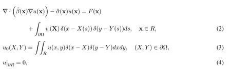
where x = (x,y) is a point in the domainR ⊃Ω ,X = (X(s),Y(s)) is a point on∂Ω assuming that∂Ω has a parametric representation∂Ω = (X(s),Y(s)).The modified source termF(x)has the following form,

The extended problem is still wellposed.The restriction of the solution ofu(x,y)on Ω is the solution to the original problem.Note that,whenβandσare constants,we use the sameβandσin the entire rectangular domainR.

2.1 Augmented IB discretization

There are variety of methods that can solve the above interface problem accurately,for example,the augmented immersed interface method.However,in this paper we wish to investigate how the IB method can be applied to solve the problem since it is straightforward,simple,and robust.

For simplification of discussion,we use a uniform mesh

assumingR=(a,b)×(c,d),whereMandN,M ∼N,are the number of the grid lines inxandydirections,respectively.The boundary∂Ω is represented by a set of ordered control points(Xk,Yk),k= 1,2,···Nb,which is then interpolated using a periodic cubic spline.We useUijto represent the finite difference approximation tou(xi,yj),Vktov(Xk,Yk),and so on.

The immersed boundary discretization then is simply the following

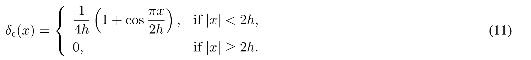
Note that,there are sophisticated discrete Dirac delta functions in the literature such as the discrete radial delta function,for example,for various purposes.Here we simply apply the original Peskin’s IB method for a first order method.

The matrix-vector form of the discretization(8),(9)can be written as

where U has the dimensionO(MN) while V has the dimensionO(Nb)∼ N,the matrixAhcorresponds to the coefficient matrix from the finite difference scheme on the rectangular domain.If we can solve the about system of linear equations simultaneously,we get a finite difference approximationUijto the original problem withO(hlogh)accuracy.

2.2 Solving the linear system of equations

If we can solve the system of Eq.(12),then we get an approximate solution to the original boundary value problems at the grid points,inside for interior problems;and outside for exterior problems.Another approach is to solve V first through the Schur complement of(12)if we apply the block Gaussian elimination method to get

whereF1is the result of the elliptic solver on the rectangular domain given the source term F1.It has been shown in Li et al.[Li and Ito(2006)]and other related papers,that the matrix-vector multiplicationSV given V is simply

whereR(V)=SV−is the residual of the boundary condition given V.More precisely,thek-th component ofSV is

whereUij’s depend on V through (10).The right hand side ofSV =can be computed from−R(0)which corresponds to the residual of the boundary condition with zero component values of the augmented variable,which is the result from the boundary value problem on the rectangular domain.Since we know how to get the matrix-vector multiplication,we can use a direct or GMRES iterative method to solve the system(13).

3 Convergence analysis

In this section we show that like the original IB method,the augmented IB method is also first order accurate except for a factor of logh.We use the exterior problem to illustrate the proof.The proof follows the path of the proof in Li et al.[Li,Zhao and Gao (1999)] for different problems.We use U and u to represent the vectors of approximate and exact solution at grid points on entireR;Tuand Eu= U−u are the vectors of the local truncation errors and the global error.We have Eu|∂Rh= 0 for the values at grid points on the boundary∂R.Similarly,we define Tqand Eq= V−v as the vectors of the local truncation error and the global error for the augmented variable in (9).According to the definitions,we have

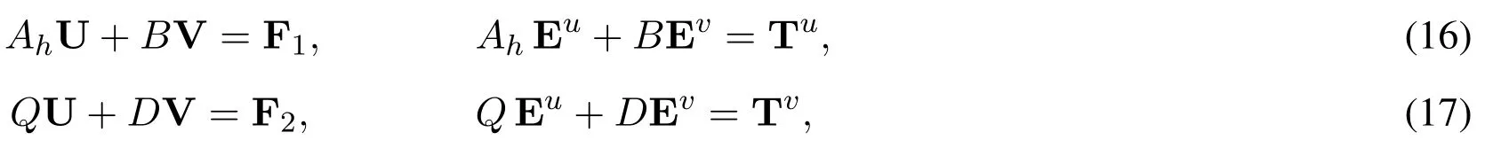
where the local truncation error vector Tuis defined as Tu=F1−Ahu−Bv and so on.

Theorem 3.1.Assume thatu(x)∈ C2(Ω),then the computed solution of the finite difference equations (8)-(9) is also first order accurate except for a factor of logh,that is,

Proof:From(16)-(17),we have

From the consistency of the interpolation formula(9),we know thatFrom the results in Li et al.[Li(2015)],we also know thatFrom the consistency of the interpolation scheme (9),we also conclude thatTherefore,now we haveSEv=U(Ev)−U(0)=O(hlogh)−0.This is because the IB method has been shown to be first order accurate except for a factor of logh.Thus,U(Ev)corresponds to the boundary value problem withu|∂R= 0 and withu|∂Ω=O(hlogh).From the maximum principle of elliptic partial differential equations,we know that the solution is also bounded byO(hlogh).Finally,the Schur complement matrixSis an interpolation scheme fromUijtoU(Xk,Yk) on the boundary.From the first order convergence and the consistency condition we haveThis completed the proof.

4 Approximation of first order partial derivatives

We also propose a simple method to find approximations of the first order derivatives at the control points on the boundary∂Ω using a one-sided interpolation.We think that with suitable choices of the parameters,the accuracy of the computed first order derivative can also be first order accurate except for a factor of logh.Note that the IB method is a smoothing method in which the discontinuity in the first order derivatives will be smoothed out.However,away from the boundary,the solution is smooth and the derivatives should be close to the true ones.We use the interior boundary value problem to explain how to compute the first order derivatives of the solution at a boundary point(Xk,Yk)to demonstrate the procedure.

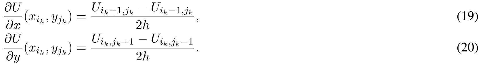
Let Xk= (Xk,Yk) be a selected point on the boundary∂Ω.We select a region Ωk:δ1,h ≤|Xk−xik,jk| ≤δ2,h,where xik,jk ∈Ω are regular grid points used (outside of the support of the discrete delta function) in the interpolation,for example,δ1,h= 3h,δ1,h= 4hor larger so that the region contains at least one grid point in the domain.The selected region should be outside of the domain where the solution will be smoothed out by the discrete delta function.We then use the standard central finite difference scheme to compute the first order derivatives

In our approach,we use the average of computed first order derivatives in the selected region,that is,

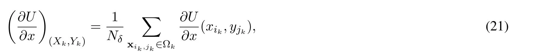
whereNδis the number of grid points in Ωk,see Fig.2 for an illustration.

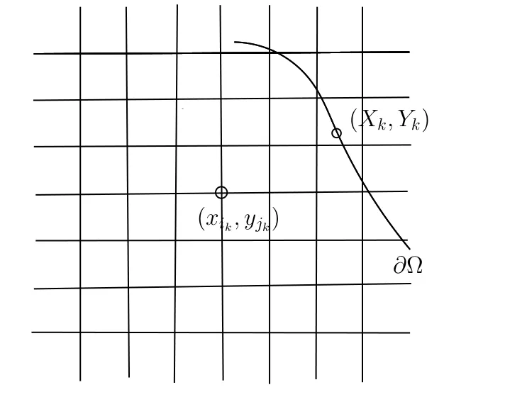
Figure 2:An illustration to compute an approximation of first order derivatives at(Xk,Yk)∈∂Ω using a regular grid point

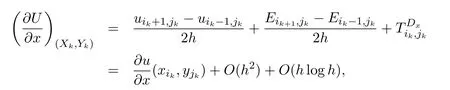
We conjecture that the computed first order derivatives are asymptotically first order convergent to the true ones at Xkwith suitable choices ofδi.Below is the sketch of the proof.We know that the computed solution is continuous,and it is smooth away from the boundary,which means

5 Numerical examples

We present a couple of numerical experiments to show the performance of the new augmented IB method for solutions and their normal derivative at the boundary.All the experiments are computed with the double precision and are performed on a MacBook Pro with Pentium(R) Dual-Core CPU,2.6 GHz,8 GB memory.We present errors in the infinity norm (pointwise).In all tables listed in this section,we useM=N=Nb.We use a constantβandσso that a fast Poisson solver based on Fast Fourier Transform(FFT)can be utilized.We use the GMRES method to solve the Schur complement system for the augmented variable with the tolerance 10−6and 0 as the initial guess in all computations.The interface is a general curve

within the rectangular domainR=[−1,1]×[−1,1].One special case is presented in Fig.1 with=0.2,L=5.

We start with aninteriorproblem withThe analytic solution is designed as

The source term and the Dirichlet boundary condition are determined from the PDE and the analytic solution.In Tab.1,we present a grid refinement analysis whenβ= 1,σ= 1.5.The second column in the table shows the maximum errors of the finite difference solution while the third column shows the ratios ofEN(u)/E2N(u) which are close to number two for a first order accurate method as we double theN.The first order convergence of solution is clearly verified.The fourth column shows the errors of the normal derivative of the solution at the boundary∂Ω pointing outward,

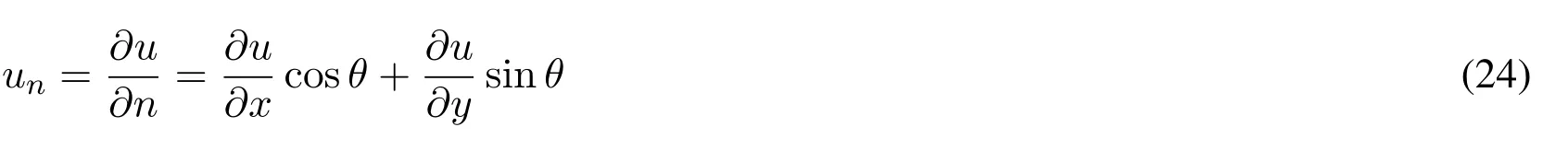
assuming the normal derivative at(Xk,Yk)is n = (cosθ,sinθ).The fifth column shows the ratios of consecutive errors which approach number two as theNgets larger.

Next we show the numerical results for anexteriorproblem with the same boundary.The analytic solution is designed as

The source term and the boundary condition are determined from the PDE and the analytic solution.In Tab.2,we present a grid refinement analysis whenβ= 2.5,σ= 1.5.We observe similar behavior as the previous example.

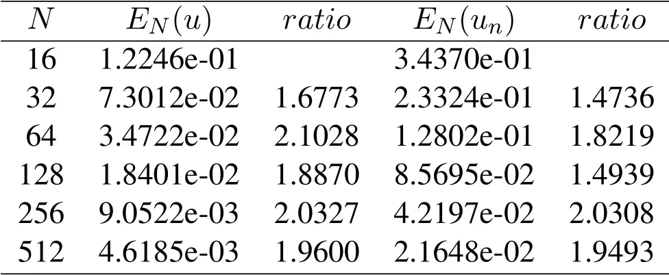
Table 1:A grid refinement analysis for the interior domain problem with σ = 1.5

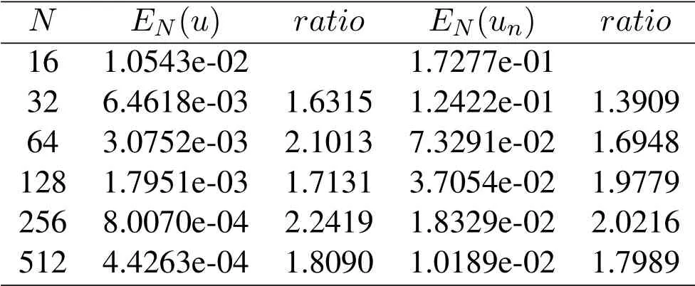
Table 2:A grid refinement analysis for the exterior domain problem with σ =1.5

As last example,we show the caseβ= 1,σ= 0,the interior boundary is simply a circler= 0.5,that is,we have a Poisson equation outside the circle.The solution isu(x,y)=sinxcosy.The grid refinement analysis results are presented in Tab.3.We can see that while the errors for the solution are smaller than that of the normal derivatives,the convergence order is roughly the same.The last column shows the number of GMRES iterations without any preconditioning techniques.In this example,the curvature is a constant and the errors behave more uniformly.

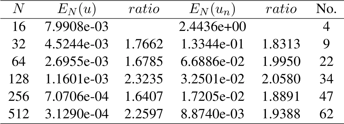
Table 3:A grid refinement analysis for the exterior domain problem with σ = 0 and a circle boundary r =0.5

6 Conclusion

In this paper,we proposed a new augmented immersed boundary method for general elliptic boundary value problems with a Dirichlet boundary condition on irregular domains.The new method inherits many properties of the original IB method for interface problems such as simplicity,robustness,and first order convergence.We also proposed a simple method to estimate first order partial derivatives which is asymptotically first order accurate.The convergence of method for the solution and the first order derivatives are also proved under appropriate regularity assumptions.How to generalize the method to other boundary conditions and how to develop efficient preconditioning techniques for the Schur complement using only the matrix and vector multiplications are two open challenges.

Acknowledgement:Z.Li is partially supported by an NSF grant DMS-1522768,CNSF grants 11871281.