
Distributed Lagrange Multiplier/Fictitious Domain Finite Element Method for a Transient Stokes Interface Problem with Jump Coefficients
2019-05-10 06:01:10AndrewLundbergPengtaoSunChengWangandChensongZhang
Andrew Lundberg,Pengtao Sun,Cheng Wang and Chen-song Zhang
1 Department of Mathematical Sciences,University of Nevada,Las Vegas,4505 Maryland Parkway,Las Vegas,NV 89154,USA.
2 School of Mathematical Sciences,Tongji University,Shanghai,China.
3 LSEC & NCMIS,Academy of Mathematics and System Science,Beijing,China.
Abstract: The distributed Lagrange multiplier/fictitious domain (DLM/FD)-mixed finite element method is developed and analyzed in this paper for a transient Stokes interface problem with jump coefficients.The semi- and fully discrete DLM/FD-mixed finite element scheme are developed for the first time for this problem with a moving interface,where the arbitrary Lagrangian-Eulerian (ALE) technique is employed to deal with the moving and immersed subdomain.Stability and optimal convergence properties are obtained for both schemes.Numerical experiments are carried out for different scenarios of jump coefficients,and all theoretical results are validated.
Keywords: Transient Stokes interface problem,jump coefficients,distributed Lagrange multiplier,fictitious domain method,mixed finite element,an optimal error estimate,stability.
1 Introduction
Let Ω be an open bounded domain in Rd(d=2,3)with a convex polygonal boundary∂Ω.Two subdomains,Ωit:= Ωi(t)⊂Ω (i= 1,2),are separated by an interface Γt:= Γ(t)which may move/deform in timet ∈[0,T](T >0),satisfyingΓt=∂Ω1t ∩∂Ω2t,as sketched in Fig.1.Then,a transient Stokes interface problem with jump coefficients can be defined as follows:
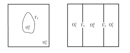
Figure 1:Two schematic domain decompositions divided by the interface Γt

where the solution pair,(u,p)that is defined in Ω×[0,T],satisfiesu|Ω1t=u1,u|Ω2t=u2,p|Ω1t=p1,p|Ω2t=p2which are associated with the source termf ∈L2(0,T;(L2(Ω))d) such thatf|Ωit=fi ∈L2(0,T;(L2(Ωit))d),(i= 1,2).The jump coefficientsβ ∈L2(0,T;L∞(Ω)) andρ ∈L∞(0,T;L∞(Ω)) satisfyβ|Ωit=βi ∈L2(0,T;W1,∞(Ωit)),ρ|Ωit=ρi ∈L∞(0,T;L∞(Ωit)),(i= 1,2),andDue to the incompressibility properties(2)and(4),we know bothρ1andρ2are constant.
It is well known that for the elliptic interface problem[Nicaise(1993);Bramble and King(1996);Boffi,Gastaldi and Ruggeri(2014);Auricchio,Boffi,Gastaldi et al.(2015)]and for the stationary Stokes interface problem[Shibataa and Shimizu(2003);Hansbo,Larson and Zahedi(2014);Olshanskii and Reusken(2006)]with jump coefficients across the interface Γt,the global regularity of solutions over the entire domain Ω are generally reduced from(H2(Ω))ddown to(H1(Ω))d,and the local regularity of solutions may be also deteriorated from (H2(Ωi))ddown to (Hσ(Ωi))d(3/2<σ ≤2) in each subdomain Ωi(i= 1,2)[Nicaise(1993)]due to a non-smooth interface Γtwhich may be only Lipschitz continuous and on which the nonzero jump fluxτmay be only defined inL∞(0,T;(Hσ−3/2(Γt))d).
The regularity study for solutions to(1)-(10)is still open to the community of theoretical partial differential equations,especially when the interface Γtdeforms along the time,i.e.,the shape of Γtand Ωit(i= 1,2) depend on the primary unknowns (u,p).In this paper,in order to show a certain amount of convergence rate during the numerical experiments process for validating the convergence theorem of the developed DLM/FD finite element method,in what follows we assume a reduced regularity result for the solution(u,p)to(1)-(10)which is similar with that of the stationary Stokes interface problem in space[Shibataa and Shimizu(2003);Hansbo,Larson and Zahedi(2014);Olshanskii and Reusken(2006)],
where,3/2<σ ≤2.Without loss of generality,in this paper we only study the immersed interface case by assuming Ω2t ⊂Ω,as shown in the left of Fig.1.The regularity property(11) is assumed to hold under the circumstance that Γtdoes not deform but only rotates and/or translates with a prescribed domain velocityw(x,t),as defined in Section 2.3.Thus the shape and position of Ωi(i= 1,2) are prescribed and do not depend on the primary unknowns,and the regularity results(11)can still be hypothesized,accordingly.Numerical results shown in Section 5 also support the regularity property of solution(u,p)defined in(11).
In practice,(1)-(10) generally model a type of immiscible two-phase fluid flow problem,where two phases of the fluid are separated by an distinct interface,and both fluid phases are defined by Stokes/Navier–Stokes equations in terms of fluid velocity and pressure as sketched in(1)-(4).In this scenario,βiandρi(i= 1,2)may stand for the fluid viscosity and density of different phases.Hence,the essential characteristic of the immiscible twophase fluid flow model is preserved in the transient Stokes interface problem(1)-(10),that is,two different types of fluid equations bearing with different viscosity and density are defined on either side of the moving interface Γt.
Some long existing body-unfitted mesh methods for interface problems such as the immersed interface method(IIM)[Deng,Ito and Li(2003);LeVeque and Li(1994);Li and Ito(2001)] and immersed finite element method (IFEM) [Li (1998);Ji,Chen and Li (2014)]are still far from satisfactory for solving the Stokes interface problem in either stationary or transient case.As for the representative body-fitted mesh method,the arbitrary Lagrangian–Eulerian (ALE) method [Hirth,Amsden and Cook (1974);Hughes,Liu and Zimmermann(1981);Huerta and Liu(1988);Nitikitpaiboon and Bathe(1993);Souli and Benson(2010)]is the most popular one for solving moving interface problems such fluidstructure interactions(FSI),where,the mesh on the interface is accommodated to be shared by both fluid and structure,and thus to automatically satisfy the interface conditions as sketched in(5)and(6).However,for large rotations and/or translations of the structure or inhomogeneous movements of the grid nodes,fluid elements tend to become ill-shaped,which reflects on the accuracy of the solution.In this case,re-meshing,in which the whole domain or part of the domain is spatially rediscretised,is then a common strategy.However,it could be very troublesome,time consuming and less accurate,and,the worst thing brought by the re-meshing is that the mesh connectivity is no longer preserved for ALE method and thus many properties of ALE method are lost.
To overcome the above problems and to deliver an efficient and accurate numerical method for the transient Stokes interface problem in which the immersed phase may be engaged in a large translational/rotational motion,in this paper we develop a body-unfitted mesh method based upon the framework of the distributed Lagrange multiplier/fictitious domain(DLM/FD) method [Glowinski,Pana,Hesla et al.(1999);Wachs (2007);Glowinski and Kuznetsov (2007);Boffi and Gastaldi (2017);Wang and Sun (2017)],where,one fluid phase is smoothly extended into the other phase that is defined in the immersed subdomain,then occupies the entire domain Ω,and the Lagrange multiplier(physically a pseudo body force) is introduced to enforce the interior (fictitious) fluids in the immersed subdomain to satisfy the constraint of the immersed phase motion.The constraints are incorporated into the field equations to form an augmented matrix equation which involves the Lagrange multipliers as unknowns.Thus,the re-meshing in the fluid domain is no longer needed for DLM/FD method,and the possible failure of ALE method is completely avoided when the large translation/rotation occurs to the immersed phase motion[Auricchio,Boffi,Gastaldi et al.(2015);Shi and Phan-Thien(2005);Yu(2005);Glowinski,Pana,Hesla et al.(2001)].The DLM/FD finite element method has been analyzed for the elliptic interface problem[Boffi,Gastaldi and Ruggeri(2014);Auricchio,Boffi,Gastaldi et al.(2015)],the parabolic interface problem[Wang and Sun(2017)],the stationary Stokes interface problem[Lundberg,Sun and Wang (2019)],but has not yet applied to the transient Stokes interface problem.As shown in Boffiet al.[Boffi,Gastaldi and Ruggeri (2014);Auricchio,Boffi,Gastaldi et al.(2015)],the DLM/FD method essentially produces a saddle-point problem in regard to the unknown of elliptic equation and Lagrange multiplier,so the existing Babuka-Brezzi’s theory [Babuška (1971);Brezzi and Fortin (1991);Brezzi (1974);Brezzi and Pitkaranta (1984)] can be employed to analyze the well-posedness,stability and convergence properties of the corresponding saddle-point problem induced from the DLM/FD finite element method.However,for the stationary Stokes interface problem,which is the steady state of the transient Stokes interface problem(1)-(10),we can see that its corresponding DLM/FD formulation forms a nested saddle-point problem including two subproblems of saddle-point type:the inside one from Stokes equations regarding Stokes unknowns (velocity and pressure),and the outside one from the DLM/FD method itself regarding Lagrange multiplier and Stokes unknowns,of which the well-posedness,stability as well as convergence analyses are more sophisticated than those of the elliptic and the parabolic interface problems.In the authors’ recent work [Lundberg,Sun and Wang(2019)],a modified DLM/FD finite element method is developed for a stationary Stokes interface problem that consists of a nested saddle-point problem,and its well-posedness,stability and optimal convergence properties are analyzed still by means of the Babuka–Brezzi’s theory but a more complicated approach.So in this paper,we will be able to develop the DLM/FD finite element method for the transient Stokes interface problem(1)-(10)and analyze its stability and convergence properties based on our previous work.
The structure of the paper is the following:in Section 2 we introduce the fictitious fluid(Stokes) equations then derive weak formulations of a transient Stokes interface problem with and without the employment of DLM/FD method.Then we define the semi-discrete DLM/FD finite element approximation and analyze its stability and optimal convergence theorem in Section 3.The full discretization is defined and its stability and convergence properties are analyzed in Section 4.Numerical experiments are carried out in Section 5,where the theoretical convergence results are validated.
2 Weak formulations of DLM/FD method
Introduce Sobolev spacesV:= (H10(Ω))d,Q:=L2(Ω),and their restrictionsV1t=Let(·,·)ωstand forL2-product inω.We also introduce the space Λt:= [(H1(Ω2t))d]∗that is the dual space of,and letdenote the duality pairing between Λtand.In Λtwe have the norm

2.1 Fictitious fluid(Stokes)equations
We first define the following Stokes equations for the fictitious fluid in Ω2tin terms of
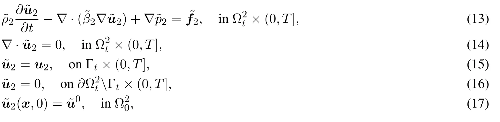
where,we smoothly extendβ1∈L2(0,T;W1,∞(Ω1t)) andρ1∈L∞(0,T;L∞(Ω1t)) into Ω2tand thus attain the continuous functionsL∞(Ω)),respectively,such thatAs a consequence,we attain a smooth functionsuch thatBecauseρ1is a constant,we assume its extension,ρ,is a constant too.In gener-Further,we introduce the solution pairsuch thatthenandAnd,a similar regularity property with(11)is defined foras well:

The following assumptions are needed in this paper:there exist constantssuch that

2.2 Weak formulations.
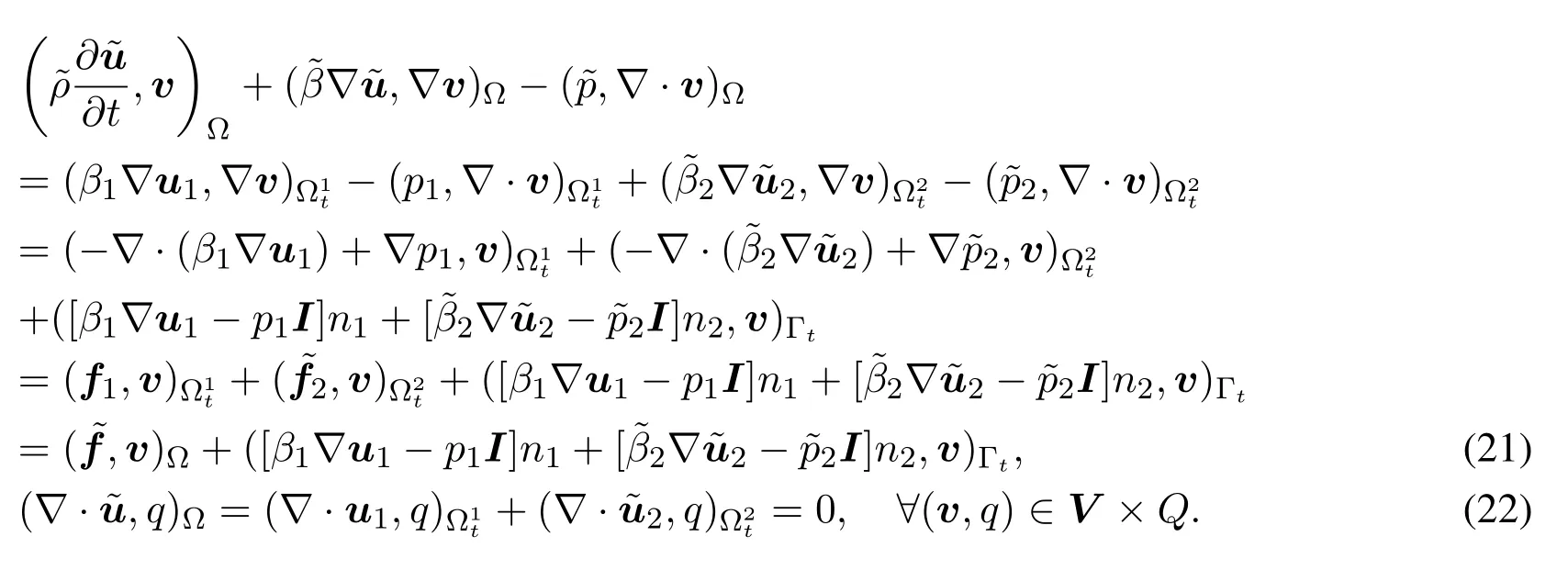
If we add the fictitious fluid Eqs.(13)-(14),which are defined in Ω2t,to the Stokes Eqs.(1)-(2),which are defined in Ω1t,and integrate by parts,then
On the other hand,if we subtract the fictitious fluid Eqs.(13)and(14)from the Stokes Eqs.(3)and(4),and integrate by parts in Ω2t,then
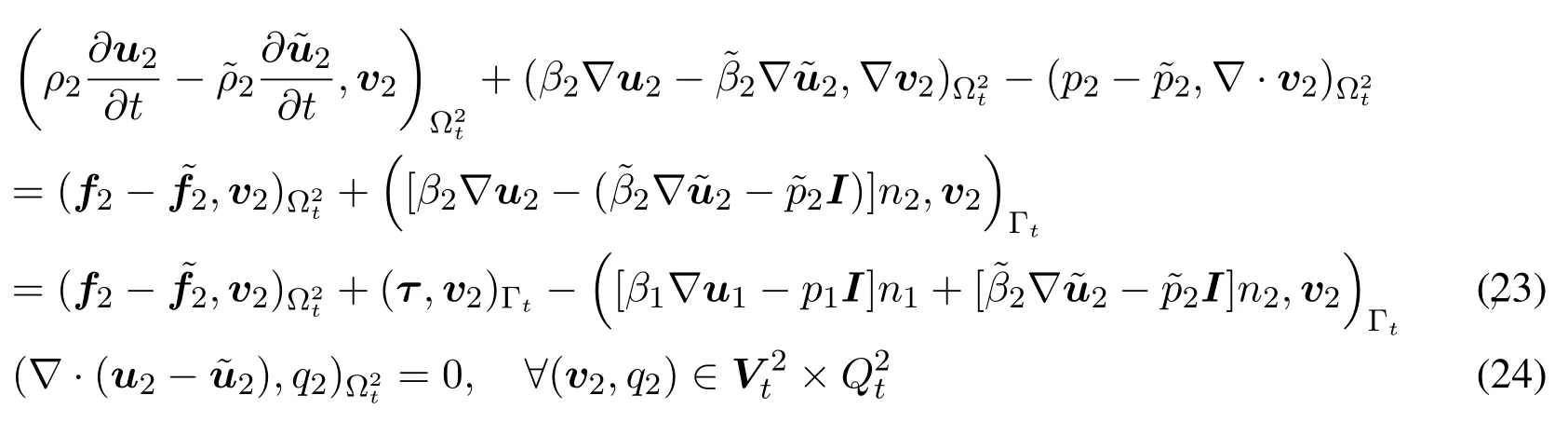
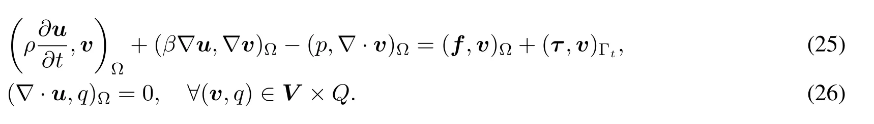
If we add (21) to (23) and (22) to (24),then the terms of the fictitious Stokes equations and the normal derivative terms on Γtare all cancelled out,resulting in the original weak formulation of(1)-(10)as follows.
Weak Form IFind(u,p)∈(H1∩L∞)(0,T;V)×L2(0,T;Q)withu|Ω1t=u1,u|Ω2t=u2,p|Ω1t=p1,p|Ω2t=p2such that
Now,we add a new constrainenforced weakly in Ω2tby means of the Lagrange multiplier,defined by

By the Fréchet-Riesz representation theorem,for eachξ ∈Λt,there exists a uniqueψ ∈V2tsuch that

where(·,·)V2trepresents theH1-inner product inV2t,defined as

In addition,(28)directly results in the following equality

Thus,(27)is equivalent with the following equation by lettingin(28)

Lemma 2.1.Let(,u2)∈H1(0,T;V)×H1(0,T;)satisfy(27)or(31),then

Proof.(32)can be easily attained by lettingin(31),then we also have

In addition,because
thus(33)is proved.Further,due to(32)

then(34)is obtained.In addition,

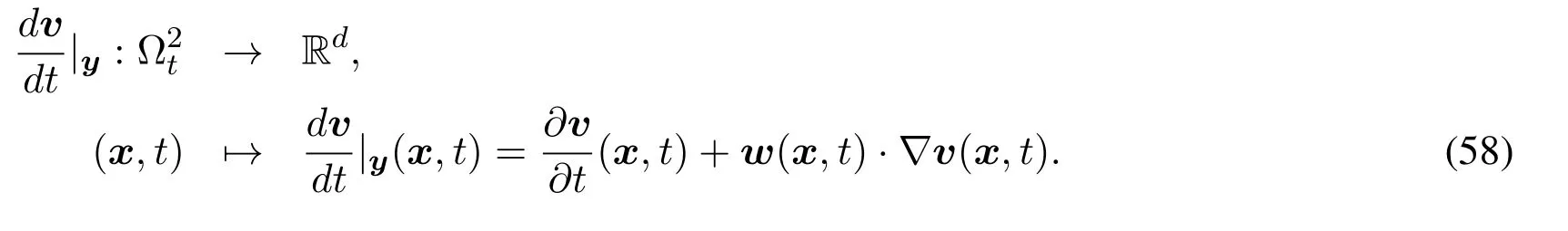
We differentiate(39)in time and apply the Reynolds transport theorem,use the prescribed domain velocity of Ω2t,w(x,t),resulting in

where,with the identity

we can further have
By the Cauchy-Schwartz inequality and(37),we obtain
choosethen(35),further,(36)are resulted,accordingly,because

With(34)and(36)we can rewrite the first and the second term on the left hand side of(23)as

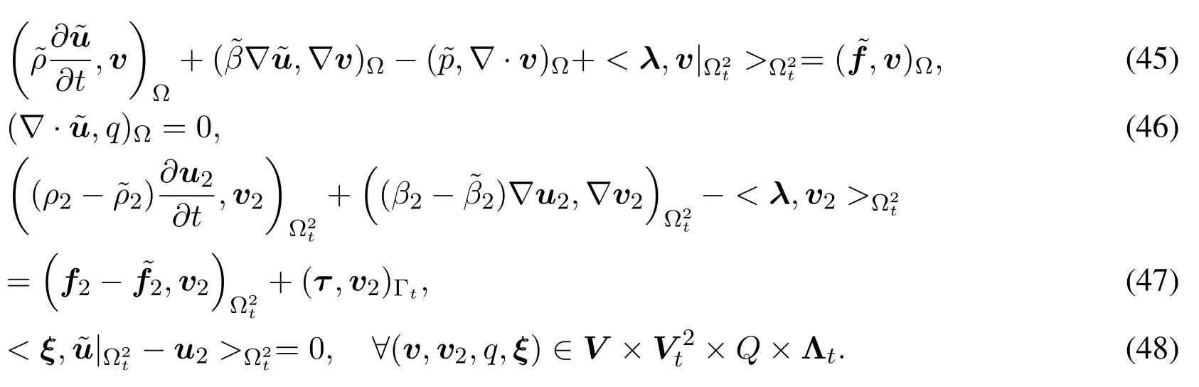
Therefore,based upon(21),(23),(26),(43),(44)and(33),we can define a DLM/FD weak formulation for(1)-(10)as follows.
Weak Form II(DLM/FD Formulation)Findsuch that
In the following theorem,we prove the equivalence between Weak Forms I and II.
Theorem 2.2.Givenandβ ∈L2(0,T;L∞(Ω))withbe any function that satisfiesand letbe any function that satisfies
(i).Suppose(u,u2,p,λ)∈(H1∩L∞)(0,T;V)×(H1∩L∞)(0,T;V2t)×L2(0,T;Q)×L2(0,T;Λt)is a solution to Weak Form II(45)-(48).LetThen(u,p)∈(H1∩L∞)(0,T;V)×L2(0,T;Q)is a solution to Weak Form I(25)and(26).
(ii).Conversely,let (u,p)∈(H1∩L∞)(0,T;V)×L2(0,T;Q) be a solution to Weak Form I(25)and(26),and defineλ ∈Λtby

Proof.(i).We have (44) due to (48) ,then (25) can be easily proved by takingv ∈Vin (45) withv|Ω2t=v2,and simply adding (45) and (47) together to cancel all Lagrange multiplier terms.Due to(33)and(46),(26)is obvious.(ii).The definition ofλ ∈Λtin(49)leads to(45),and
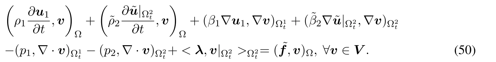
Subtract (50) from (25),(47) is then obtained becauseu|Ω2t=u2that is the selection of the solution,(48) is thus proved as well.Due to (33) and (26),(46) is obvious by takingq ∈Qwith
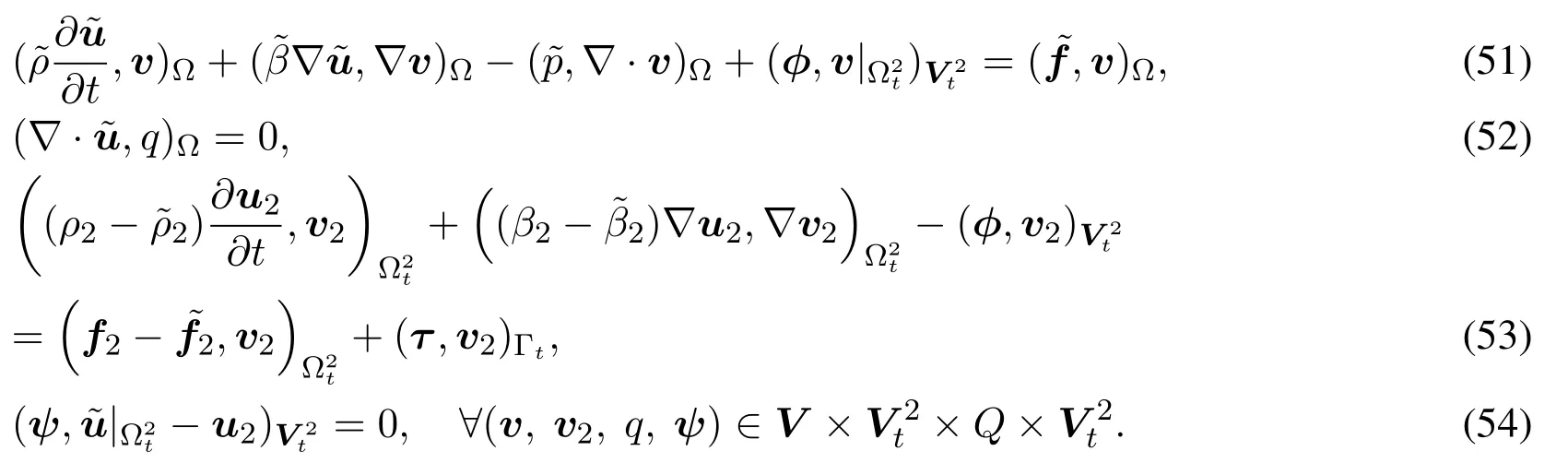
According to the equivalence of (27) and (31),we can reformulate the weak forms of DLM/FD method as follows.
Weak Form III (Equivalent DLM/FD Formulation)Findsuch that
2.3 The arbitrary Lagrange-Eulerian(ALE)formulation
We assume that there exists a bijective mappingXt ∈H1(0,T;(W2,∞(Ω20))d)such that for eacht ∈(0,T],the mapping[Martín,Smaranda and Takahashi(2009);Gastaldi(2001)]
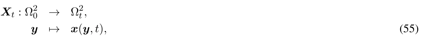
is invertible andHerey ∈Ω20is so called the arbitrary Lagrange-Eulerian(ALE)coordinate,andx ∈Ω2tis the spatial(or Eulerian)coordinate.We further introduce the domain velocityw,defined by

In this paper we assume that Ω2tdoes not deform but only rotates/translates with a prescribed domain velocity,w.Thus,w(x,t)∈H1(0,T;(W1,∞(Ω2t))d)is a given velocity function with the assumption that

wherecdenotes a constant independent of any discretization parameters in the rest of the paper.so the ALE mapping functionXt(y,t)∈H1(0,T;(W2,∞(Ω20))d),which can be considered as a prescribed displacement of domain motion for Ω2t.
Now we need to redefine the spaceon the ALE frame as follows:where,is the reference(initial)domain of.Based on the above definitions,we can reformulate(51)-(54)as the following ALE-type weak formulation of the DLM/FD method.
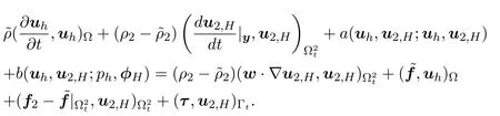
Weak Form IV(ALE-DLM/FD Formulation)Findsuch that
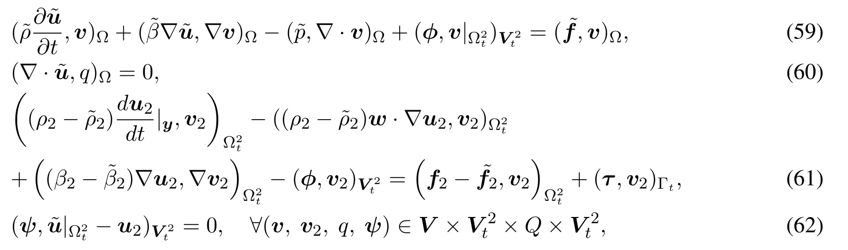
where,we introduce a convection term((ρ2−)w·∇u2,v2)Ω2tin(61).The main technical reason to introduce this term is strictly numerical.Since the domain is time dependent,it is not possible to discretize directly the partial temporal derivative.In fact,if x ∈Ω2tand the time step size ∆t >0,the condition x ∈Ω2t+∆tis not always fulfilled.Therefore,the term((ρ2−)w·∇u2,v2)Ω2tcould be seen as a numerical corrector term of the partial temporal derivative.
3 Semi-discretization of DLM/FD finite element method
Let Th(Ω) be a partition of Ω with the mesh size h that is independent of the location of the interface Γt,and let TH(Ω2t)be a partition of Ω2twith the mesh size H,where,H can be different from h.Based on these two meshes,we can introduce the conforming finite element space to each continuous space as:Considering the limited regularity results(18),one possible choice of finite element spaces is the following
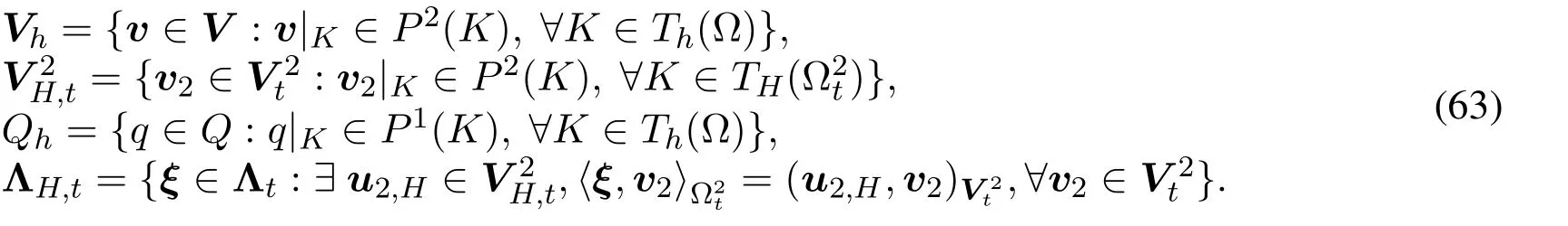
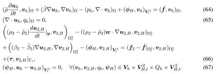
where,Vh ×Qhis a stable pair ofP2P1mixed (Taylor-Hood) finite element space for Stokes equations.In fact,it is proved in [Lundberg,Sun and Wang (2019)] that such chosen mixed finite element spacesfor a fixed timetis stable for the developed DLM/FD method for the stationary Stokes interface problem–the steady state case of the transient Stokes interface problem(1)-(10).Thus,based upon the DLM/FD weak form III (51)-(54),is still adopted as the stable mixed finite element spaces for the DLM/FD finite element method of(1)-(10),as defined below.Find(uh,u2,H,ph,φH)∈(H1∩L∞)(0,T;Vh)×(H1∩L∞)(0,T;V2H,t)×L2(0,T;Qh)×L2(0,T;V2H,t)such that
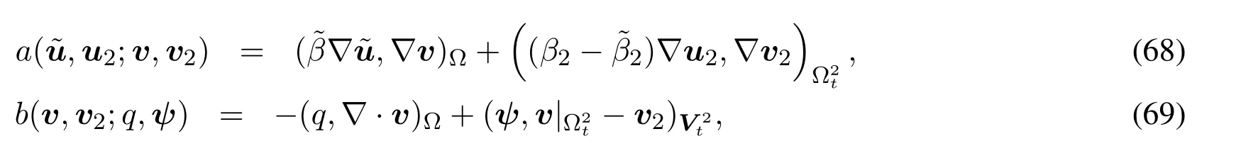
To analyze the convergence and stability properties of the semi-discrete finite element approximation(64)-(67),we first introduce the following bilinear forms for an ease of deduction:
and define the discrete divergence-free space as

Then we know(uh,u2,H)
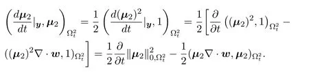
Let (zh,z2,H,χh,θH) be arbitrary functions inand letη=φ−θH,γ=θH−φH.Takevh=µ,v2,H=µ2in(64)-(67),subtract(64)-(67)from(59)-(62)and consider(52),(54),(65),(67)and(58),yields

Reynolds transport theorem leads to the following formula
Further,apply the factb(µ,µ2;ξ,γ)=0 and Young’sε−inequality to(70),we obtain
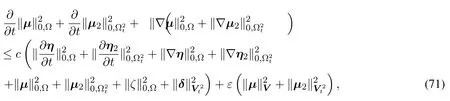
where,we use conditions(19),(20)and(57).Addt o both sides of(71),choose a sufficiently smallε,then take integral on both sides of(71)with respect to time from 0 tot,yields
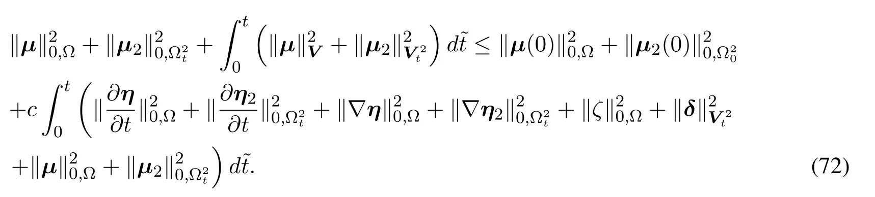
Apply the Grönwall’s inequality,leads to
Then,we have the following convergence theorem for the semi-discretization(64)-(67).
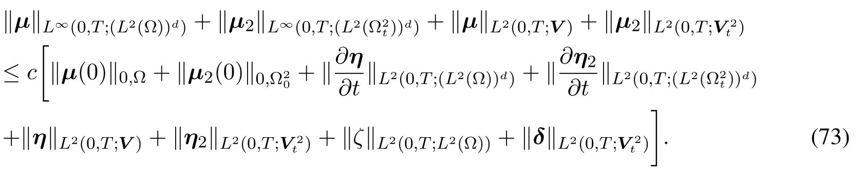
Theorem 3.1.Suppose(,u2,p,φ)is the solution to(59)-(62),(uh,u2,H,ph,φH)is the solution to (64)-(67).WithP2-P2-P1-P2mixed finite element to respectively discretizeuh,u2,H,ph,φH,we have the following error estimate
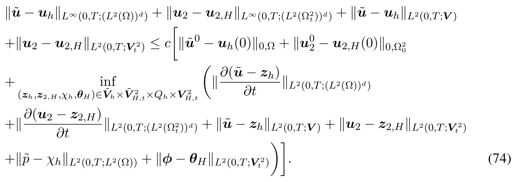
Note that on the right hand side of(74),all terms butcan be directly estimated based on a priori interpolation error estimates and the regularity assumptions(18).To find an error estimate forwe first pick anyv ∈Vin(51)such thatv=0 outside Ω1tincluding∂Ω1t.Integrating by parts gives

Similarly,we can pick (v,v2)∈V ×V2tsuch thatv|Ω2t=v2andv= 0 outside Ω2tincluding∂Ω2t.Add(51)to(53)and integrate by parts,yields

Now,letv ∈Vand takeAdd(51)to(53),we have

where the integrals over Ω are split into Ω1tand Ω2t.Integrating by parts,yields

then apply(75)and(76),we attain

Further,apply(76)and(79)to(53),and note thatn1=−n2,we have
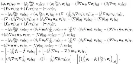
We can writeφ=φ1+φ2+φ3+φ4,where

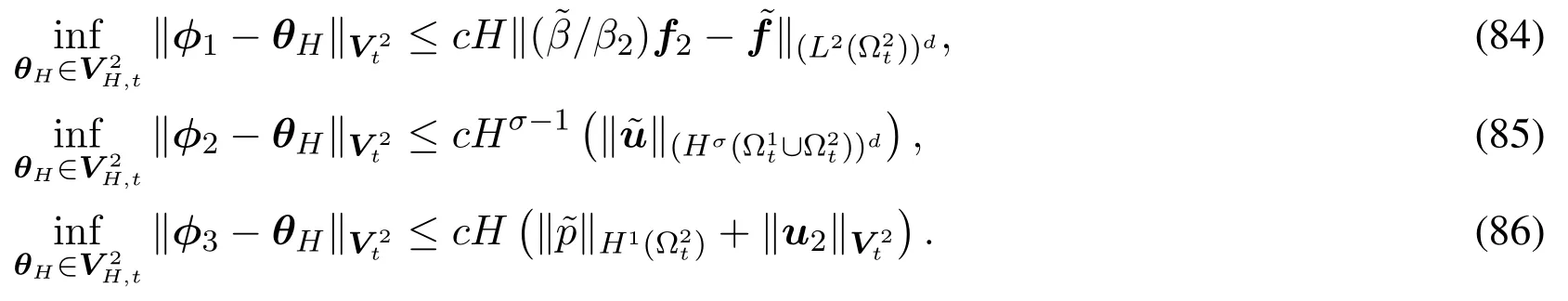
With the regularity assumptions (18),we can obtain the following estimates by doing an analogous analysis with[Auricchio,Boffi,Gastaldi et al.(2015);Lundberg,Sun and Wang(2019)]whilet ∈(0,T]is temporarily fixed,

It is easy to see thatOn the other hand,because of the choice of finite element space (63),our finite elementsV2H,tand ΛH,tare contained inL2(Ω2t),we can interpret the duality pairing as scalar product inL2(Ω2t)[Auricchio,Boffi,Gastaldi et al.(2015);Boffi,Gastaldi and Ruggeri (2014)].Thus,we can definePHλ4∈ΛH,tbe theL2-projection ofλ4onto ΛH,tsuch that
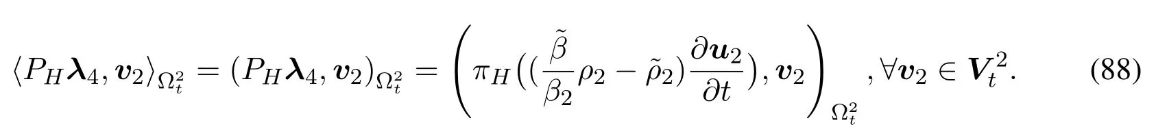
So by(87)we havefor allv2∈V2H,t.Then,
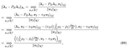
where,we apply (87) and (83).By applying the Cauchy–Schwartz inequality and the a priori interpolation error estimate forπH,we obtain

Then there exists a constantc>0 such that

Combine(84)-(86)and(91),we obtain the error estimate ofdisplayed as
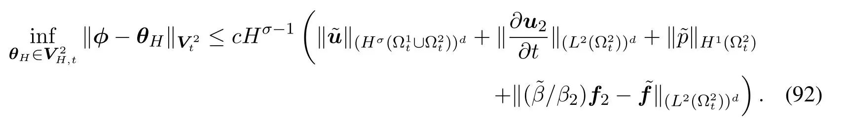
Together with the a priori interpolation error estimates forand takewhereπh:V →Vhandare appropriately defined interpolation operators.Then we attain the following a priori error estimates for the semi-discrete DLM/FD finite element method of the transient Stokes interface problem.
Theorem 3.2.Letbe the solution to(59)-(62),and letbe the solution to (64)-(67).If (19),(20)and(57)hold,then there exists a constantc>0 independent ofhandHsuch that

Now we analyze the stability property of the semi-discrete scheme.Takevh=uh,v2,H=u2,Hin(64)-(67),yields
Note thatb(uh,u2,H;ph,φH)=0,apply Reynolds transport theorem and Young’sε−inequality,and use(19),(20)and(57),results

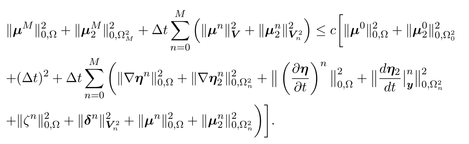
where,the trace estimate is applied to getIntegrate both sides of(93)in time from 0 tot,addto both sides,choose a sufficiently smallε,and apply Poincaré inequality in Ω and Grnwall’s inequality to(93),reads
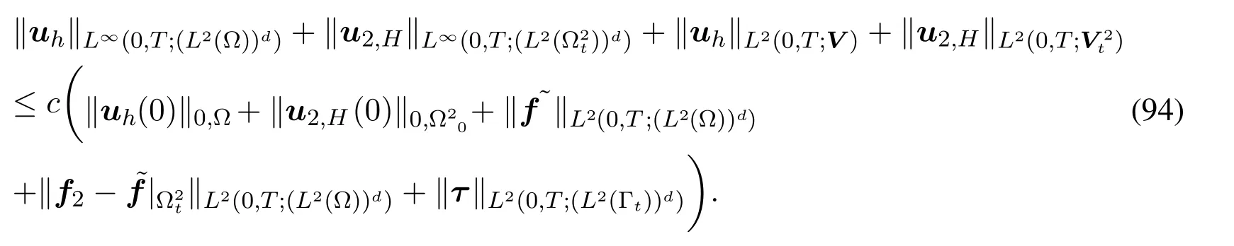
Then,we have the following stability theorem for the semi-discrete scheme.
Theorem 3.3.Suppose all hypotheses of Theorem 3.1 are held,then the stability result(94)exists for(64)-(67).
4 Full discretization of DLM/FD finite element method
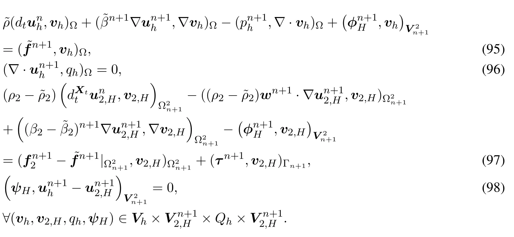
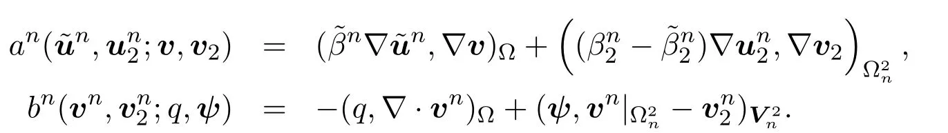
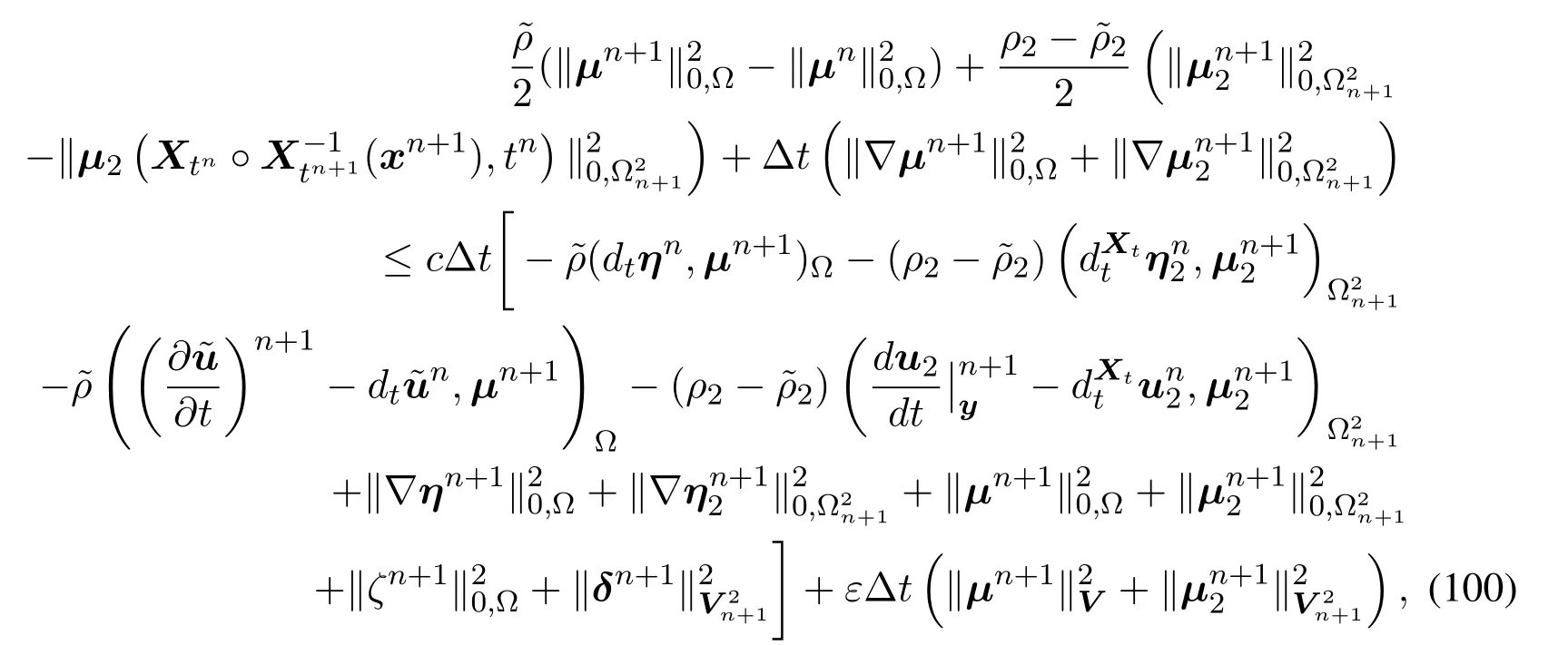
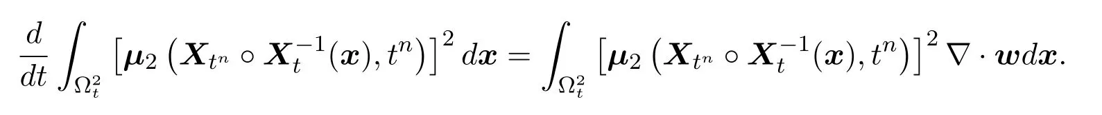
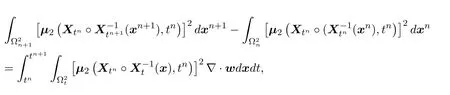
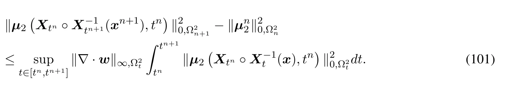
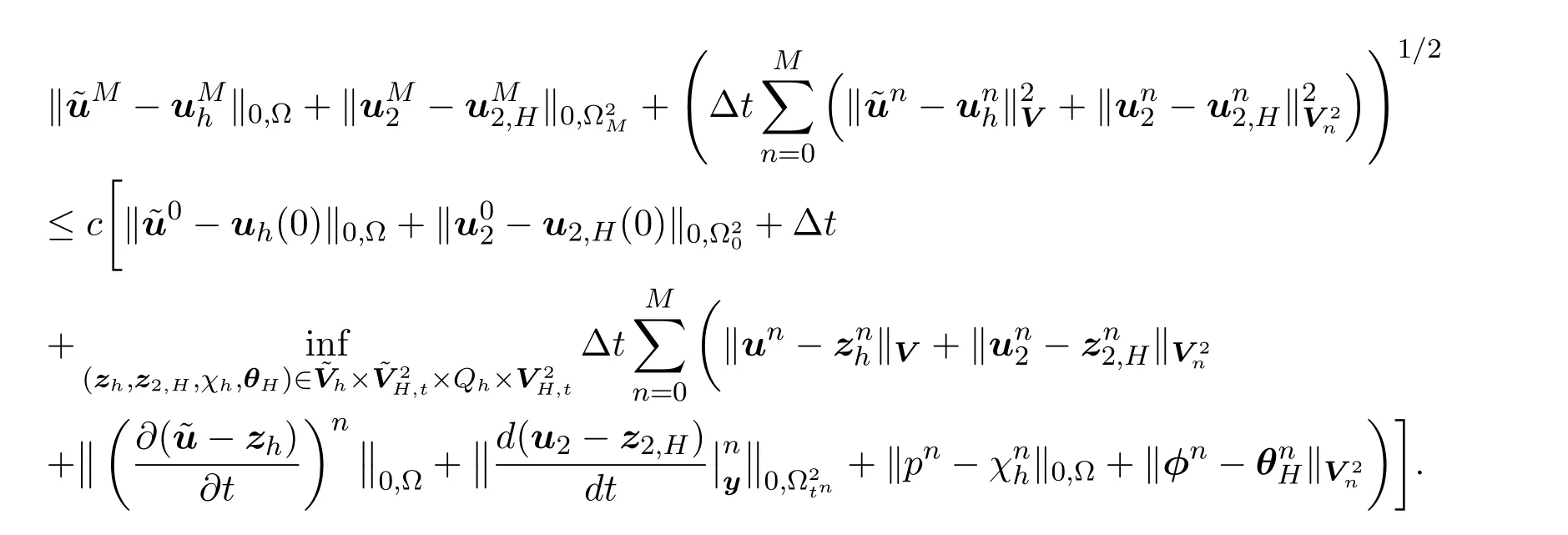
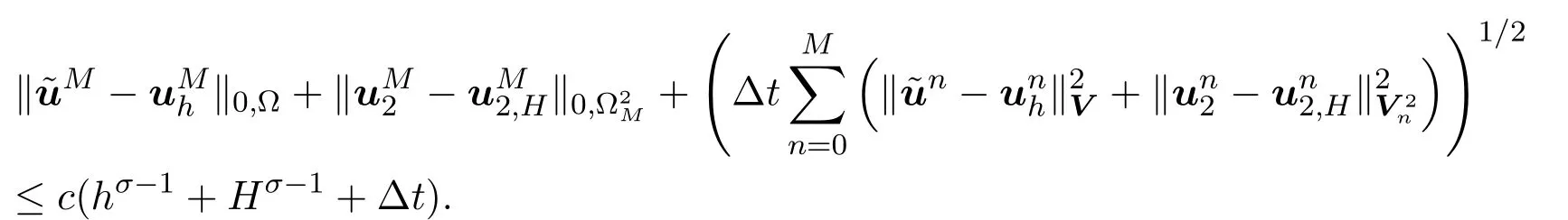
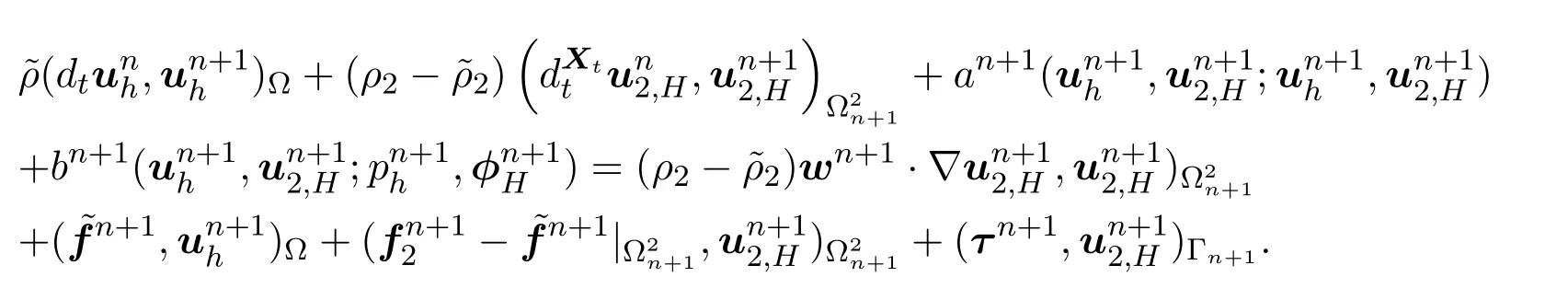
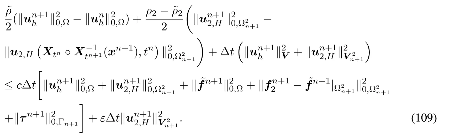
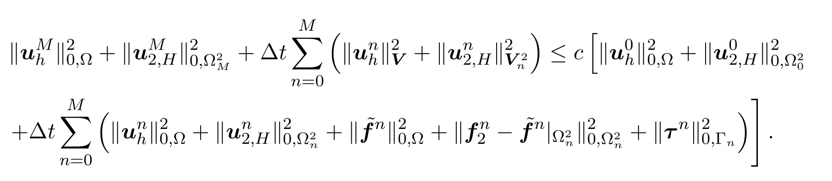
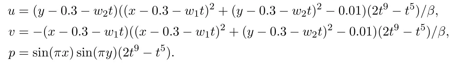
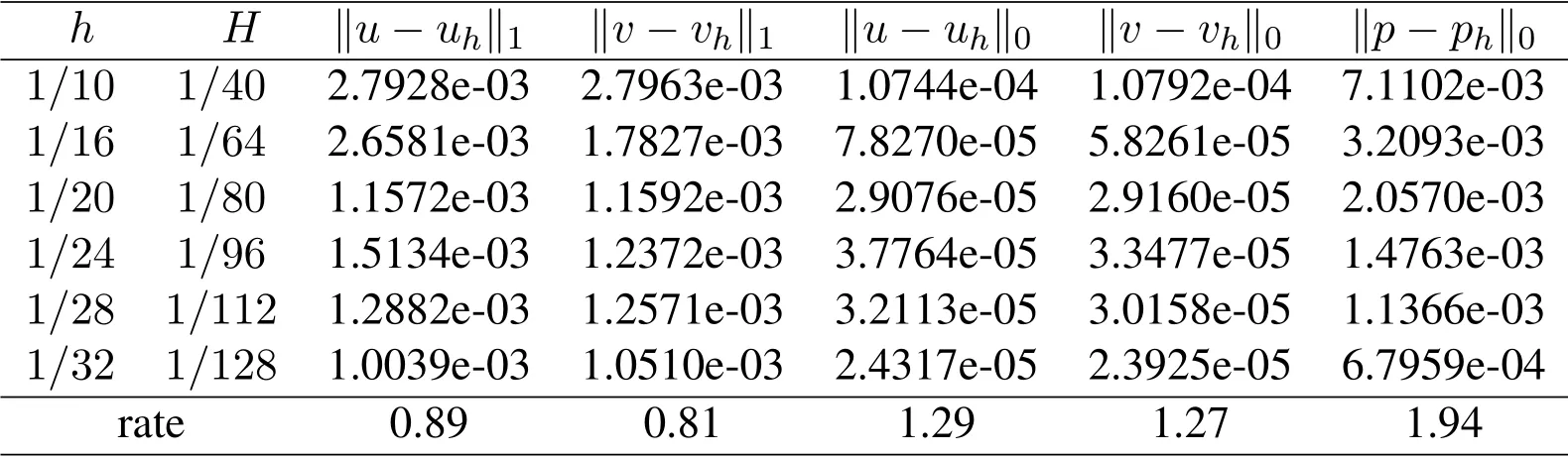
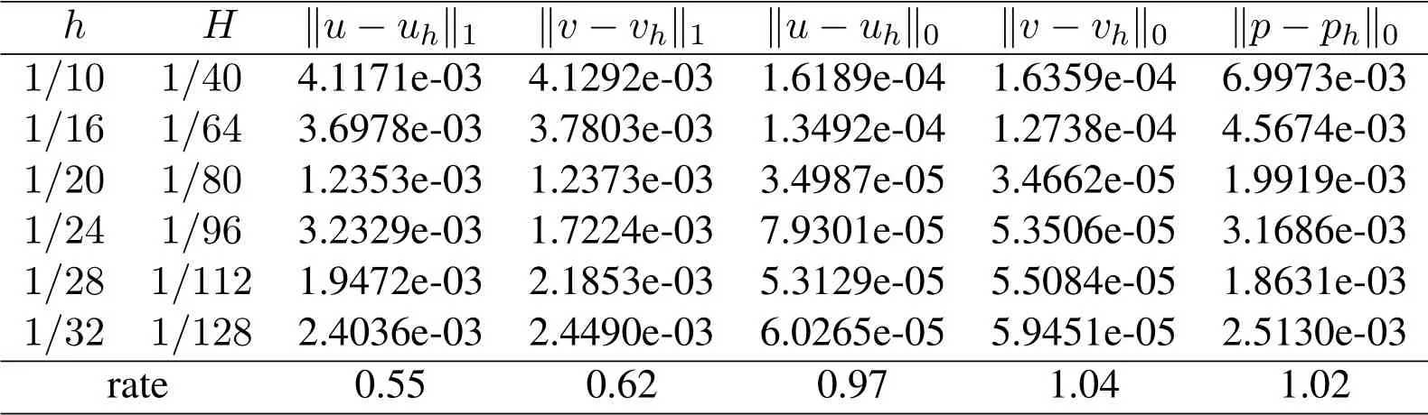
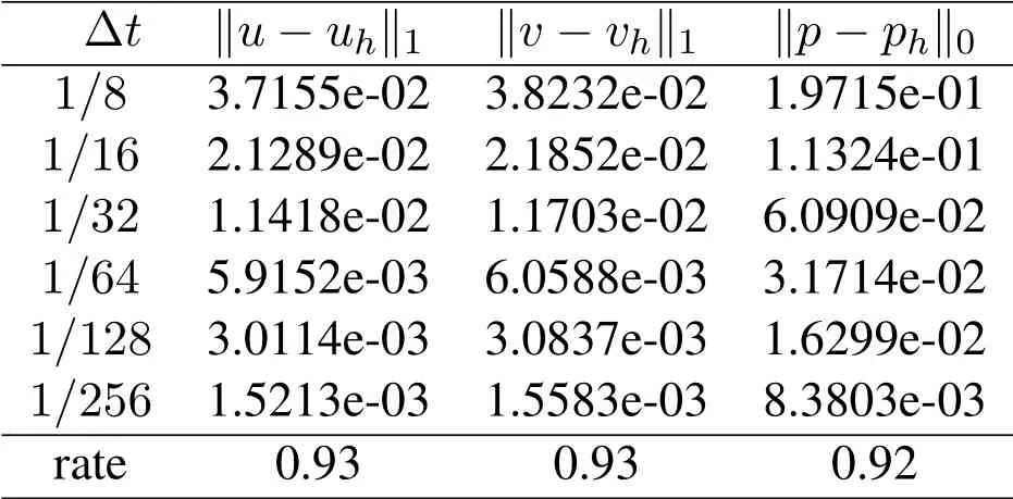
Introduce a uniform partition 0 =t0 Attn,we particularly letTn2,Hbe a partition of Ω2n:= Ω2tnwith the mesh sizeH,and letbe the conforming finite element space defined onTn2,H.And,we still letThbe a partition of Ω with the mesh sizehthat is independent of the location of the interface Γn:=Γtn.Then,the full discretization of DLM/FD finite element approximation for(59)-(62)can be defined as:forn=0,1,··· ,N−1,supposeunh ∈Vandun2,H ∈V n2,Hare known,findsuch that Introduce the following bilinear forms attn: Now we analyze the error estimate of the full discretization (95)-(98) by letting (zh,z2,H,χh,θH)be arbitrary functions inis the discrete divergence-free space attn+1.With the same notations in Section 3,we have the following error equation by subtracting(95)-(98)from(59)-(62), Takevh=µn+1,v2,H=µn+12in(99),noticebn+1(µn+1,µn+12;ξn+1,γn+1) = 0,and apply(19),(20),(57)and Young’sε−inequality,we obtain where,we need to further analyze the termon the left hand side of(100).By the Reynolds transport theorem,we know Integrate fromtntotn+1,yields namely, In order to bound the last temporal integral,due to the change of variablez=Xtn(X−1t(x)),we have[Martín,Smaranda and Takahashi(2009)] where,Jdenotes the determinant of Jacobian matrix which are bounded since the one-toone functionXtis prescribed.Together with(57),(101)leads to Then,(100)can be further rewritten as Based on Taylor’s expansions,the following inequalities can be derived: where,denotes the second partial temporal derivative on the ALE frame,and the assumption(57)is used. Sum up both sides of (104) overnfrom 0 toM−1 (M= 1,··· ,N),apply Taylor’s expansions(105)-(108)and choose sufficiently smallε,yield Then we have the following error estimate Consider the regularity assumptions(18),adopt the same approximation to the initial valuesu0andu02as done in Section 3,and apply(92),then the following convergence theorem is derived for the fully discrete DLM/FD scheme(95)-(98). Theorem 4.1.Letbe the solution to (59)-(62),and letbe the solution to(95)-(98).If(19),(20)and(57)hold,then there exists a constantc >0 independent ofhandHsuch that The stability of the full discretization is studied as follows.Takein(95)-(98),yields Apply (103) to the termon the left hand side of(109),then sum up both sides of (109) overnfrom 0 toM−1 (M= 1,··· ,N),apply Taylor’s expansions(105)-(108),choose sufficiently smallε,yield Apply the discrete Grönwall’s inequality,results Then,we have the following stability theorem for the fully discrete scheme. Theorem 4.2.Suppose all hypotheses of Theorem 4.1 are held,then the stability result(110)exists for(95)-(98). In this section,we study the numerical performance of the developed DLM/FD finite element method for an example of the transient Stokes interface problem(1)-(10)defined inΩ= [0,1]×[0,1],where the circular subdomain Ω2tmakes a translational motion and the position of∂Ω2t,which is the interface Γt,satisfies where,w=(w1,w2)Tdenotes the moving velocity of Γt. We properly choose the functions of coefficients,source terms and jump flux of(1)-(10),i.e.,βi,ρi,fi,(i= 1,2) andτsuch that the true solution (u,p) to (1)-(10),whereu=(u,v)T,is defined by where,β=βi(x),∀x ∈Ωi(i= 1,2) is chosen as a piecewise constant depending on the location ofx.Clearly,such chosen solution (u,p) satisfies the following regularity property: In what follows,we take a constant moving velocityw=(0.1,0.2)T,and letT=1.The meshesTh(Ω)andTH(Ω2t)are constructed independently and thus mismatched with each other. Convergence results of the velocity vector at the timet=Tin itsH1-andL2norm,i.e.,which are displayed in their component forms,and of the pressure in itsL2norm,,are illustrated in Tabs.1 and 2 for large jump coefficient cases.We can observe that:(1)the developed DLM/FD–mixed finite element discretization is stable and converges in all cases,little influence from the choice of the time step size;(2)the convergence results are relatively more sensitive toβ2/β1,comparing with the jumpρ2/ρ1,noting that the exact solutionudepends onβ,but independent ofρ;(3)due to the reduced regularity property of the solution,and the discontinuity of the normal derivative ofuacross Γt,the convergence rates of velocity errors inH1- andL2-norm decrease to 0.55∼0.9 and 1.0∼1.3,respectively,and the convergence rates of pressure errors inL2-norm keeps around 1.0∼2.0,which validate our theoretical conclusions,and also match with the convergence rates of other types of interface problems when the DLM/FD method is applied[Boffi,Gastaldi and Ruggeri(2014);Auricchio,Boffi,Gastaldi et al.(2015);Wang and Sun(2017);Lundberg,Sun and Wang(2019);Sun(2019)]. Next,we investigate the influence of time step size on the convergence rate of the developed DLM/FD finite element method.In order to letO(∆t) be the main part of the error in comparison with the partO(hσ−1+Hσ−1),we particularly pick up the case ofβ2/β1=2,ρ2/ρ1= 2,and takefi,(i= 1,2) andτsuch that the true solution (u,p) to (1)-(10),whereu=(u,v)T,is defined by Numerical results of this test are reported in Tab.3,from which we can observe the firstorder convergent for all errors with respect to ∆t,as predicted by the theoretical result. Table 1:Convergence results of the case: β2/β1 =100,ρ2/ρ1 =1000,∆t=1/128 Table 2:Convergence results of the case: β2/β1 =10000,ρ2/ρ1 =1000,∆t=1/128 Table 3:Convergence results of the case: β2/β1 =2,ρ2/ρ1 =2,h=1/32,H =1/128 We develop the DLM/FD–mixed finite element method for a generic transient Stokes interface problem and carry out numerical analyses for both semi-and fully discrete scheme on the convergence and stability properties.By using the Taylor-Hood (P2P1) mixed finite element space,we are able to obtain a nearly optimal convergence rate for both the velocity and the pressure in their respective norms,subjecting to the reduced regularity assumption for the solution to the transient Stokes interface problem.Numerical experiments validate the theoretical results,showing that the convergence rates of the velocity with respect to the mesh size is the 0.5th inH1-norm,and the first order inL2-norm,at least,which is true even for larger jump coefficient cases up to 1:10000,relatively insensitive to different choices of jump coefficients and time step sizes.And,the first order convergence rate with respect to the time step size is also validated. Acknowledgement:P.Sun was supported by NSF Grant DMS-1418806.C.S.Zhang was partially supported by the National Key Research and Development Program of China (Grant No.2016YFB0201304),the Major Research Plan of National Natural Science Foundation of China(Grant Nos.91430215,91530323),and the Key Research Program of Frontier Sciences of CAS.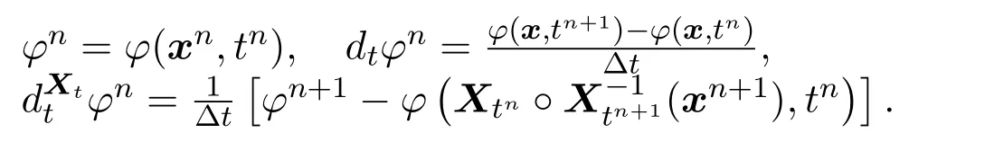


5 Numerical experiments


6 Conclusion and future work
 Computer Modeling In Engineering&Sciences2019年4期
- Computer Modeling In Engineering&Sciences的其它文章
- Computational Modeling of Human Bicuspid Pulmonary Valve Dynamic Deformation in Patients with Tetralogy of Fallot
- Convergence Properties of Local Defect Correction Algorithm for the Boundary Element Method
- A Novel Image Categorization Strategy Based on Salp Swarm Algorithm to Enhance Efficiency of MRI Images
- An Immersed Method Based on Cut-Cells for the Simulation of 2D Incompressible Fluid Flows Past Solid Structures
- Multiscale Hybrid-Mixed Finite Element Method for Flow Simulation in Fractured Porous Media
- An IB Method for Non-Newtonian-Fluid Flexible-Structure Interactions in Three-Dimensions