A modified logarithmic spiral method for determining passive earth pressure

Shiyi Liu,Yng Xi,Li Ling

aSchool of Resources and Civil Engineering,Northeastern University,Shenyang 110819,China

bState Key Laboratory of Structural Analysis for Industrial Equipment,School of Automotive Engineering,Dalian University of Technology,Dalian 116024,China

Keywords:Passive earth pressure Logarithmic spiral method Finite element method(FEM)Sloping back fill Retaining wall

A B S T R A C T In this study,a modified logarithmic spiral method is proposed to determine the passive earth pressure and failure surface of cohesionless sloping back fill,with presence of wall-soil interface friction.The proposed method is based on a limit equilibrium analysis wherein the assumed profile of the back fill failure surface is a composite of logarithmic spiral and its tangent.If the wall-soil interface is smooth,a straight line does not need to be assumed for the failure surface.The geometry of the failure surface is determined using the Mohr circle analysis of the soil.The resultant passive earth thrust is computed considering equilibrium of moments.The passive earth pressure coefficients are calculated with varied values of soil internal friction angle and cohesion,wall friction angle and inclination angle,and sloping back fill angle.This method is verified with the finite element method(FEM)by comparing the horizontal passive earth pressure and failure surface.The results agree well with other solutions,particularly with those obtained by the FEM.The implementation of the present method is efficient.The logarithmic spiral theory is rigorous and self-explanatory for the geotechnical engineer.

1.Introduction

Passive earth pressure plays an essential role in design of geotechnical engineering structures such as retaining walls,antisliding piles and bridge abutments.Different approaches,e.g.limit equilibrium methods such as the Coulomb(1776)and Rankine(1857)theories,as well as limit analysis and numerical analysis,have been proposed to calculate the passive earth pressure.The Rankine and Coulomb theories still serve at present as the fundamentals of this subject(Terzaghi et al.,1996;Budhu,2010;Braja and Khaled,2014).The Rankine(1857)theory assumes that the resultant force is angled parallel to the back fill surface.Once the back fill surface is horizontal,the assumption indicates that the wall-soil interface should besmooth(i.e.thewall friction angle equal to zero).Such an assumption is not adopted in the Coulomb(1776)theory,because Coulomb’s equation of passive earth pressure has been extended to account for wall friction.However,the planar failure surface assumption in the Coulomb theory may not be suitable in the case of a larger wall friction angle as it could overestimate the passive earth pressure.Despite these drawbacks,the theory has been widely used and accepted by engineers due to its simplicity.

Terzaghi(1943)noted that the failure surface shouldbe curved if the wall-soil interface is rough(i.e.the wall friction angle is larger than zero).For this,he proposed a method known as the logarithmic spiral method,which is one of the earliest methods used to describe the passive limit equilibrium of a sliding mass moving along a curved failuresurface.After that,a composite failure surface comprising a logarithmic spiral and its tangent was adopted in different limit equilibrium methods(Shields and Tolunay,1972;Zhu and Qian,2000;Kumar,2001;Rao and Choudhury,2005;Shamsabadi et al.,2013;Patki et al.,2015a).The logarithmic spiral failure mechanism(i.e.the failure surface of merely a logarithmic spiral)can be studied using the limit equilibrium method(Patki et al.,2015b)and kinematical method(Soubra and Macuh,2002).

The slip-line field theory,a powerful mathematical technique,can be used to solve plane strain boundary value problems in plasticity domain.This theory provides exact solutions to rigid plastic solids(Bower,2010).The slip-line method(the method of characteristics)(Sokolovskii,1965;Kumar and Chitikela,2002;Cheng,2003)does not need to assume the shape of failure surface;however,it is helpful for understanding the behaviour of a soil-wall system and the failure mechanism.But in practice,it is difficult to solve a particular problem using this method as finding out the slip-line field is rather difficult.

Fig.1.Logarithmic spiral method for determining the passive earth pressure(Terzaghi,1943;Terzaghi et al.,1996).(a)Model of a gravity wall retaining horizontal back fill under vertical surcharge loading;(b)Free body that is divided into the logarithmic spiral zone and the Rankine zone;(c)Forces for computation of component due to the weight of soil,while neglecting the cohesion and surcharge loading;(d)Forces for computation of component due to the vertical surcharge loading,while neglecting the weight of soil and cohesion;(e)Forces for computation of component due to the cohesion,while neglecting the weight of soil and surcharge loading;(f)Lateral forces acting on the Rankine zone;(g)Vertical surcharge Q;and(h)Diagram illustrating computation of the moment due to cohesion.

Limit analysis,which is based on the upper and lower bound theorems of classical plasticity,is another common method used to determine passive earth pressures.It is easy to obtain the upper limit of passive earth pressures with upper bound solution(Chen,1975;Soubra and Regenass,2000;Soubra and Macuh,2002;Antão et al.,2011).However,it is difficult to construct statically admissible stress fields in the lower bound analysis(Shiau et al.,2008).To overcome this difficulty,the finite element limit analysis is proposed(Sloan,2013).

Finite element analysis is a popular tool used to evaluate geotechnical structure stability,e.g.slope engineering(Griffiths and Lane,1999;Liu et al.,2015).The finite element method(FEM)has been widely used for calculation of passive earth pressures(e.g.Tejchman et al.,2007;Hanna et al.,2011;Hanna and Diab,2017).Under certain conditions(e.g.wall-soil contact),the finite element analysis is more efficient and can yield more reasonable result with respect to slope failure mechanism.

Terzaghi(1943)developed the logarithmic spiral method;unfortunately,few studies have been reported on this method.This is likely due to the implementation difficulty.Based on the logarithmic spiral method developed by Terzaghi,we proposed a modified method for calculations of passive earth pressures and failure surfaces.In the modified method,the shape of the failure surface for a smooth wall is not assumed as a straight line.The modified method can determine the passive earth pressure and failure surface of a cohesionless sloping back fill.The passive earth pressure coefficients are evaluated for various values of soil friction angle φ,soil cohesionc,wall friction angleδ,sloping back fill angleβand wall inclination angleλ,and then they are compared with existing results.Then,the feasibility of the method is verified by the FEM.

Fig.2.Mohr circle analysis for determining the Rankine zone.(a)Stresses of an element in a sloping back fill and the failure pattern;and(b)Passive stress analysis of soil.

2.Formulation of logarithmic spiral method

2.1.Principle

It is assumed that the soil satisfies the Mohr-Coulomb failure criterion,which is expressed as follows:

whereτandσare the shear stress and normal stress on the failure surface,respectively;andcand φ are the cohesion and internal friction angle,respectively.In the logarithmic spiral method,the internal friction angle φ of soils(not the cohesionc)governs the shapes of the failure surface and the spiral.

Fig.1 illustrates the passive earth pressure problem of retaining wall,which can be solved using the logarithmic spiral method(Terzaghi,1943;Terzaghi et al.,1996).Moment equilibrium conditions are employed to calculate the magnitude of passive thrust.It is assumed that the failure surface comprises a logarithmic spiral and a tangent surface.The resultant passive earth pressurePpis decomposed in to three components:P1,P2andP3.Each of these forces acts at an angleδ(the wall friction angle),normal to the contact faceab.P1maintains force equilibrium due to the weight of the massabgfand the friction,P2maintains force equilibrium due to the vertical surcharge load acting on the horizontal back fill surface and the friction,andP3maintains force equilibrium with the cohesion on the sliding surface.

The soil within the triangleageis in the passive Rankine state.The failure surfacebgecomprises a logarithmic spiral partbgand a straight partge(Terzaghi,1943;Terzaghi et al.,1996).In polar coordinates(r,θ),the logarithmic spiral part is determined by

where e is the base of natural logarithm,andr0and φ are the random positive real constants(φ is also the soil internal friction angle).For the logarithmic spiral,the angle φ is constant between the line perpendicular to tangent direction and the radial line at the point(r,θ).This indicates that as the size of the spiral increases,its shape will not be altered upon each successive curve.The straight partgeof the failure surface is tangent to the spiralbgat the pointg,and thus the pole of the spiral must be located on the rayga.Note that the location of the pole is different from that assumed by Terzaghi et al.(1996),who suggested that the pole is located on lineag.Assumption of a different location of pole would yield a considerable difference in the calculation results.

The body force of soilabgfis used to conduct the moment equilibrium analysis,and the following forces act onabgf:three forcesP1,P2andP3;soil weightW;resultant forceQinduced by the vertical surcharge loadingq;the momentMcinduced by the cohesion alongbg;the componentsPRW,PRQ,andPRCof the resultant thrust of the Rankine passive earth pressure,which are angled parallel to the back fill surface;and the resultantF1andF2of the normal and frictional stresses alongbg(Terzaghi,1943;Terzaghi et al.,1996).Because the moments induced byF1andF2at poleOare zero,the equations of the moment equilibrium can be expressed as:

whereyfis they-coordinate of the pointf.Thex-coordinatexfcan be written asxf=yftanα2.

The momentMcof the total cohesion alongbg(Terzaghi et al.,1996)is calculated as follows:

The resultant passive earth pressurePpcan be defined as follows:

It is noted that the failure surface corresponds to the resultant forcePpas determination of the passive earth pressure using the logarithmic spiral method becomes an optimization problem.Ppis the objective function andyfis the design variable(Terzaghi,1943;Terzaghi et al.,1996).It is important that the defined domain ofyfshould be specified by the user with experiences to a reasonable range.In this paper,yfis an arithmetic progression and the common difference in the successive members is selected as small as possible.

2.2.Logarithmic spiral failure surface

The logarithmic spiral cannot be described based on the concept of the logarithmic spiral method proposed by Terzaghi(1943)and Terzaghi et al.(1996).An approximate method is proposed herein to determine the shape and location of the logarithmic spiral.

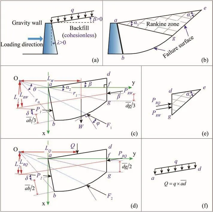
Fig.3.Modified logarithmic spiral method for determining passive earth pressure in the case of inclined cohesionless back fill.(a)Model of gravity wall retaining a sloping back fill under vertical surcharge loading;(b)Free body divided into the logarithmic spiral zone and Rankine zone;(c)Forces entering into computation of component due to the weight of soil,neglecting the vertical surcharge loading;(d)Forces entering into computation of component due to the vertical surcharge loading neglecting the weight of soil;(e)Lateral forces acting on the Rankine zone;and(f)Vertical surcharge Q.

Fig.4.A finite element grid for the passive earth pressure analysis.Materials of the foundation and back fill are the same.

As shown in Fig.1c,d and e,in the Cartesian coordinate systemxay,the coordinates of pointsaandbare considered as variables.They-coordinate of pointfis the same as that of the pointg.xOrepresents thex-coordinate of the poleO,and they-coordinate of the poleOis obtained by the following equation:

For a given value of they-coordinate of pointf(i.e.yf),xOcan be obtained by solving the following equations:

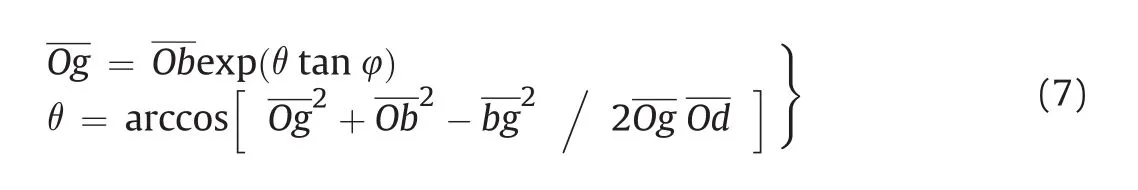
whereθis the corresponding angle of the logarithmic spiralbg(see Fig.1c).The logarithmic spiralbgcan be described by functionθ(yf).Eq.(7)can be solved with root- finding algorithms using the bisection method.This solution is implemented by a proposed numerical code implemented in MATLAB.

2.3.Passive Rankine zone

As shown in Fig.1b and f,the shape of the triangular Rankine zone can be determined by the anglesα1and α2.In the case of a horizontal back fill surface(β =0°),these two angles would be the same,i.e.α1= α2= π/4- φ/2.

In general,in the case ofβ ≠ 0°,the angles α1and α2are determined with the Mohr circle analysis.As shown in Fig.2a,the vertical stressσvof the soil elementabcdat a depth ofzis obtained by the following equation:

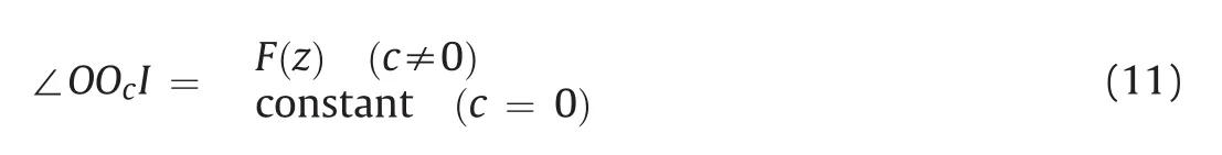
whereγis the weight of soils,andqis the vertical surcharge loading.In the analysis of Mohr circle for a two-dimensional state of stress(Fig.2b),it is assumed that the length of lineOIis equal to the vertical stress of the soil elementabcd,i.e.OI=σv.We can draw a parallel line from pointIto the σvplane of stress acting;alternatively,a parallel line from pointMto theσhplane of action can be plotted.The intersection of any two lines with the Mohr circle is the poleN.The angle betweenOIand thex-axis is the same as the sloping back fill angleβ.According to the geometric figure,∠OOcIcan be solved by the following equations:

Eq.(9)can also be expressed as follows:

The solution to Eq.(10)is given:

whereFis a function of the heightz.The anglesα1and α2are expressed as follows:

Fig.5.Results of(a)the horizontal passive earth pressure coefficient and(b)failure surface(contours of displacement after time step=3)using the finite element method.The solid black line(i.e.the failure surface)obtained with the logarithmic spiral method is used for the comparison with the contours from the finite element method.

Fig.6.Results of the passive earth pressure and failure surfaces obtained by the logarithmic spiral method for φ =40°.

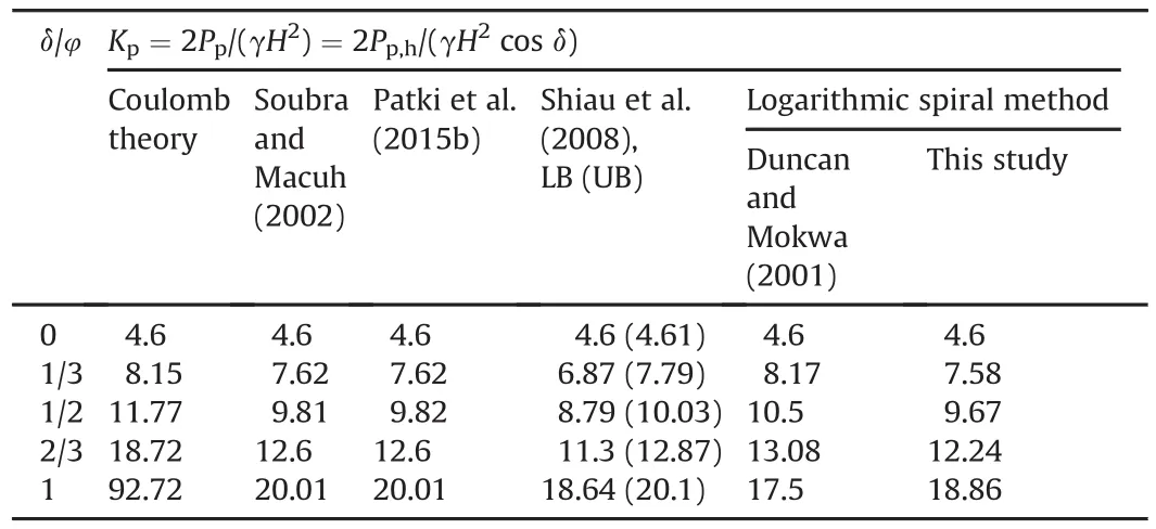
Table 1 Results comparison(φ =40°).

Table 2 Comparison of the results obtained by the numerical limit analysis and the logarithmic spiral method.

However,Eqs.(11)and(12)show that the anglesα1and α2vary with depth whenc≠ 0 andβ≠ 0°.This indicates that the logarithmic spiral method cannot effectively address the problem of cohesive sloping back fill.Thus future study is needed.

As shown in Fig.2b,in the case of cohesionless sloping back fill,c=0,the angle∠OOcIcan be expressed as follows:

Substituting Eq.(13)into Eq.(12)yields

The Rankine passive earth pressure coefficientKpR(Rankine,1857)is expressed as follows:

Fig.3 provides the solution for determining the passive earth pressure with the modified logarithmic spiral method in the case of inclined cohesionless back fill.

Fig.7.Comparison of the results obtained by the numerical limit analysis and logarithmic spiral method.LB and UB represent the lower and upper bounds,respectively.

3.Finite element modelling

A back fill is assumed with a heightH=5 m that is retained by a rigid gravity wall.The materials of the foundation and back fill are the same,which is shown in Fig.4.A 45°edge cut is introduced to benefit the numerical solution(Shiau and Smith,2006).The elastoplastic finite element analysis for determining the passive earth pressure is achieved using ABAQUS(Smith,2010).The CPE4R element(i.e.a 4-node bilinear plane strain quadrilateral,reduced integration element)is adopted to discretize the finite element model.Passive failure is induced by pushing the rigid retaining wall into the soil back fill.The bottomedge of the foundation is fixed.The right-and left-hand edges of the foundation and the right-hand edge of the back fill are fixed in the horizontal direction.Vertical movement of the wall is not allowed.A displacement is applied to the right of the nodes at the left edge of the gravity wall.

The retaining wall is assumed to be linearly elastic with Young’s modulus of 20.3 GPa,Poisson’s ratio of 0.2 and density of 2500 kg/m3.The back fill and foundation are assumed to be elastic-perfectly plastic.The elastic response of the soil is assumed to be linear and isotropic,with Young’s modulus of 182MPa,Poisson’s ratio of 0.3and density of 2040.8 kg/m3.The soil back fill follows Mohr-Coulomb behaviour with associated flow rule.The linear Drucker-Prager yield criterion is adopted for simulation of the soil back fill in the numerical analysis due to its smoothyield surface. The constitutive model parameters can be matched to provide the same flow and failure response in the plane strain condition(Helwany,2007;Smith,2010).The following relationships provide a match between the Mohr-Coulomb and linear Drucker-Prager material parameters in the plane strain condition:

wheredis the intercept of the linear yield surface,andψis the dilation angle in thep-qstress plane(pis the equivalent stress andqis the Mises equivalent stress).Considering the case of associated flow,ψ = β,we obtain

An example is given to show the finite element solution for determination of the passive earth pressure.Fig.5a shows the relationship of the horizontal passive earth pressure coefficientKp,hwith the time step of the finite element analysis for the case of φ =40°and δ/φ =1/2.The asymptotic limiting value corresponds to the maximumKp,hthat could be mobilized.Fig.5b shows the variation in the contour of displacement with time step.The solid black lines are the slip surface obtained by the logarithmic spiral method.The results show that the failure surfaces obtained with the two methods are the same after the 3rd time step.

Fig.8.Comparison of horizontal passive earth pressure distributions on smooth and rough walls for various values of φ.

4.Results and discussion

The passive earth pressure and failure surface of a rigid retaining wall were obtained by the modified logarithmic spiral method under a wide range of variables,e.g.variations in geometry,wall soil interface and soil back fill properties.The results are compared with existing results and that of the FEM.

4.1.Typical results

Fig.6 shows the magnitudes of the passive thrust and critical failure surfaces obtained with the logarithmic spiral method at φ =40°with varied wall friction angle.The basic assumption with respect to the failure surface is that the shape of the failure surface is convex.For the smooth wall,the radian of the failure surface below the spiral zone(i.e.the region above the logarithmic spiral curve)is approximatelyπand the coordinate of the pole of the spiral failure surface is approximately(-∞,+∞).Therefore,the failure surface of the spiral zone is roughly a straight line.

TheKpvalues obtained by the logarithmic spiral method are reported in Table 1,in comparison with the results from other methods.For rough walls(δ/φ ≠ 0),the logarithmic spiral method by Duncan and Mokwa(2001)predicted higher values ofKpthan our results,except for the fully rough case(δ/φ =1).The numerical upper and lower bounds obtained by Shiau et al.(2008)are close to our results and the results of Soubra and Macuh(2002)and Patki et al.(2015b);however,our results are the lowest.

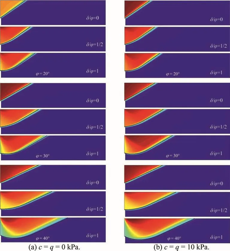
Fig.9.Comparison of failure surfaces obtained by the finite element method(contour of displacement)and logarithmic spiral method(solid black line)for various values of φ.

More generally,analyses are performed for various values of soil internal friction angle φ.A comparison between the results obtained by the numerical limit analysis(Shiau et al.,2008)and the logarithmic spiral method is presented in Table 2 and Fig.7.The numerical upper and lower bounds match our results,except for the fully rough case(δ/φ =1)with φ ＞ 30°,whereKpvalues are closed to and even smaller than the lower bound.The reason accounting for this discrepancy in the fully rough case(δ/φ =1)with φ＞30°remains unclear;however,verification with the FEM result might be an alternative to provide insight into the accuracy of the logarithmic spiral method.

Figs.8a and 9a show the results obtained by the modified logarithmic spiral method and FEM for the cohesionless back fill at various values of φ.In Fig.8a,the distributions of the earth pressure in the middle of the walls,obtained using the two methods,are basically the same.Difference between the boundary nodes near the top and bottom of the wall may be caused by the stress concentration and the horizontal direction being fixed on the left edge of the foundation in the finite element analyses.As shown in Fig.9a,thefailure surfaces of the two methods are essentially the same(i.e.the shapes and locations of the failure surfaces are in good agreement).

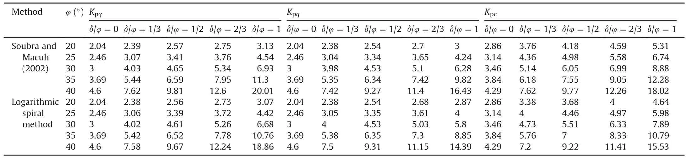
Table 3 Comparison of proposed Kpγ,Kpqand Kpcvalues with the results from Soubra and Macuh(2002).

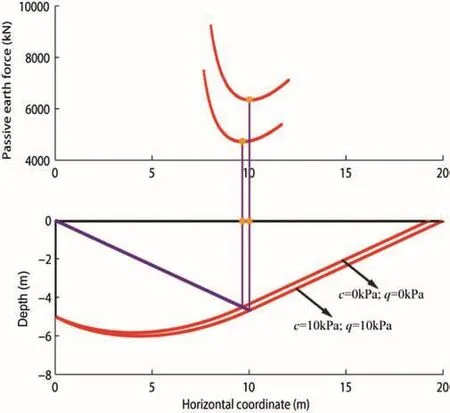
Fig.10.Comparisons of failure surface and passive earth pressure obtained by the logarithmic spiral method for c=q=0 kPa and c=q=10 kPa(φ = δ=40°).

4.2.Effect of cohesion

For the cohesive back fill retained by a vertical wall and loaded by vertical surcharge loading,the passive force is expressed as follows:

whereKpγ,KpqandKpcare the passive earth pressure coefficients and represent the effects of soil weight,vertical surcharge loading and cohesion,respectively(Soubra and Macuh,2002).Kpγiscalculated with the assumption of cohesionless soil without surcharge loading.The computation of the coefficientsKpqandKpcis based on the assumption of weightless soil withc=0 kPa forKpqandq=0 kPa forKpc(Soubra and Macuh,2002).Based on the definitions ofKpγ,KpqandKpc,Table 3 compares our results with those obtained by Soubra and Macuh(2002).Our results are close to or less than the results from Soubra and Macuh(2002),suggesting that the results are the upper bound obtained from the kinematical approach(Soubra and Macuh,2002)and different assumptions of failure mechanism are adopted.

Table 4 Passive earth pressure coefficients Kpγ-log,Kpq-logand Kpc-logwhen φ = δ=40°.

Fig.11.Comparison of the horizontal passive earth pressure coefficient with the results obtained by finite element limit analysis(Shiau et al.,2008).

The passive force calculated by Eq.(19)would be less than or equal to the true value.In other words,the passive earth pressure coefficients are not constant in the case of cohesive back fills under vertical surcharge loading.In the logarithmic spiral method,the passive earth pressure coefficientsKpγ-log，Kpq-logandKpc-logare expressed as follows:

whereP1+P2+P3=P.Table 4 shows the passive earth pressure coefficientsKpγ-log，Kpq-logandKpc-logobtained by the logarithmic spiral method when φ = δ=40°with variousγ,candqvalues.The coefficientsKpqandKpcbased on the assumption of a weightless soil withc=0 forKpqandq=0 forKpc,andKpγcalculated with assumption of cohesionless soil without surcharge loading are the minimum values ofKpγ-log,Kpq-logandKpc-log.

Fig.12.Comparison of horizontal passive earth pressure distributions for various values ofβ (φ =30.9°,and δ=19.2°).

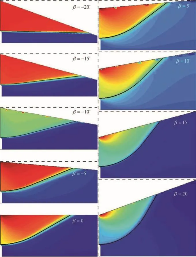
Fig.13.Comparison of the failure surfaces obtained by the finite element method(contour of displacement)and the logarithmic spiral method(solid black line)for various values of β (φ =30.9°,and δ=19.2°).

Figs.8b and 9b show the results obtained by the logarithmic spiral method and FEM for cohesive back fills under vertical surcharge loading with various values of φ.Similarly,the same distribution of earth pressure is observed in the middle of the wall.The failure surfaces obtained by the two methods are essentially the same.Furthermore,considering the effects of cohesion and surcharge loading,the critical failure surface is deeper,and the magnitude of the passive thrust is larger than that without consideration of the effects of cohesion and surcharge loading(Fig.10).

4.3.Effect of back fill slope

This example is taken from the work of Shiau et al.(2008)(φ =30.9°,δ=19.2°,λ=0,c=q=0)to examine the feasibility of the logarithmic spiral method with various values of the back fill slope angleβ.Fig.11 shows the comparison of horizontal passive earth pressure coefficients obtained by numerical limit analysis and the logarithmic spiral method.The upper and lower bounds are close to the results of the logarithmic spiral method with the angleβ increasing from-10°to 20°.In addition,the horizontal passive earth pressure coefficients whenβ=-20°andβ=-15°are proposed using the logarithmic spiral method.

Figs.12 and 13 show the results of the horizontal passive earth pressure distributions and failure surfaces based on the logarithmic spiral method and FEM using various values ofβ,respectively.In Fig.12,the same distribution of earth pressures is observed in the middle of thewalls except whenβ=-20°,where a slight difference is observed.As shown in Fig.13,the failure surfaces based on the two methods are essentially the same(i.e.the shapes and locations of the failure surfaces agree well).The failure surface changes from plane(β =-20°)to curved(β =-15°to-20°)and the size of the ground surface of the passive sliding body reduces when the angle is increased from-20°to 20°.

Fig.14.Forces used in computation of component due to weight of soil and friction for the concave failure mechanism(Kumar,2001).

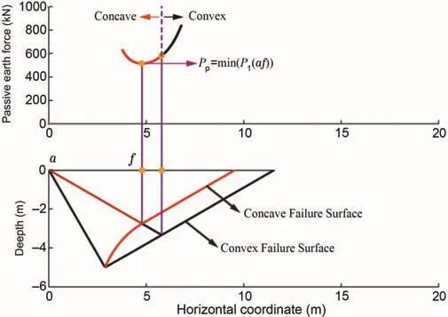
Fig.15.Comparisons of failure surface and passive earth pressure obtained by the logarithmic spiral method for convex and concave failure mechanisms(φ =30°,δ/φ =0,and λ=30°).

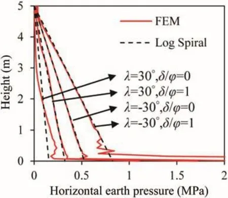
Fig.16.Comparison of horizontal passive earth pressure distributions for various values ofλ(φ =30°).

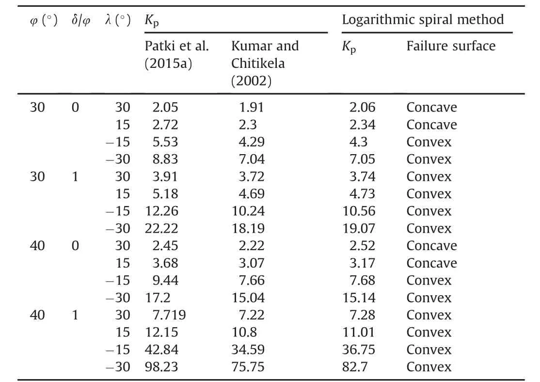
Table 5 Comparison of proposed Kpvalues with those obtained by other methods for inclined retaining wall with horizontal cohesionless back fill.

4.4.Effect of wall inclination

Kumar(2001)studied the effect of wall inclination on passive earth pressure coefficients for cohesionless soil and proposed a concave failure mechanism(see Fig.14).When φ =30°,δ/φ =0,and λ =30°,Fig.15 shows the comparisons of critical failure surface and magnitude of passive thrust accounting for both convex and concave failure mechanisms.The failure surface corresponding to the minimum magnitude of the passive thrust is concave.A comparison of the passive earth pressure coefficients with those obtained by other methods is shown in Table 5.The results obtained by the logarithmic spiral method are greater than those obtained by Kumar and Chitikela(2002)and less than those from the limit equilibrium method by Patki et al.(2015a).In addition,for the case of smooth walls(δ/φ =0),the failure surfaces are concave for both λ=30°and λ=15°.

Fig.17.Comparison of failure surfaces obtained by the finite element method(contour of displacement)and the logarithmic spiral method(solid black line)for various values ofλ(φ =30°).

The FEM is used to verify the assumption of a concave failure mechanism.Taking φ =30°as an example,Figs.16 and 17 indicate the distribution of horizontal passive earth pressure and failure surface forλ= 30°,δ/φ =0 and 1,respectively.The failure surfaces obtained by the two methods agree with each other,except when λ =30°and δ/φ =0.In Fig.17,the concave failure mechanism is unreasonable,and the corresponding horizontal passive earth pressure distribution is not a graded distribution,as shown in Fig.16.However,the corresponding passive earth pressure coefficient is generally accurate for practical design.

5.Conclusions

A modified logarithmic spiral method is proposed to determine the passive earth pressure coefficients and failure surfaces.The passive earth pressure coefficients are calculated at various values of soil internal friction angle and cohesion,wall friction angle and inclination angle,and sloping back fill angle.Then,these coefficients are compared with the existing results.Finally,the method is verified with the FEM with respect to the horizontal passive earth pressure and failure surface.The main conclusions are drawn as follows:

(1)The logarithmic spiral method developed by Terzaghi et al.(1996)is modified in this context.It is demonstrated that the modified method is efficient,which can be used to determine the passive earth pressure and failure surface of a cohesionless sloping back fill.

(2)The results obtained from our modified method agree well with other solutions,in particular those obtained by the FEM.

(3)The logarithmic spiral theory is rigorous and self explanatory for the geotechnical engineer.

The modified logarithmic spiral method presented in this study still has some limitations.One major problem is that it cannot be used to accurately solve problems involving cohesive sloping back fill,which needs future studies.

Conflicts of interest

The authors wish to confirm that there are no known conflicts of interest associated with this publication and there has been no significant financial support for this work that could have influenced its outcome.

Acknowledgements

This work is funded by the Doctoral Scientific Research Foundation of Liaoning Province(Grant No.20170520341)and the Fundamental Research Funds for the Central Universities(Grant No.N170103015).These supports are gratefully acknowledged.