Influence of data analysis when exploiting DFN model representation in the application of rock mass classification systems

Tkko Miyoshi,Dvide Elmo,*,Steve Rogers

aNBK Institute of Mining,University of British Columbia,Vancouver,Canada

bGolder Associates Ltd.,Vancouver,Canada

Keywords:Data collection Discrete fracture network(DFN)Classification system Geological strength index(GSI)

A B S T R A C T Discrete fracture network(DFN)models have been proved to be effective tools for the characterisation of rock masses by using statistical distributions to generate realistic three-dimensional(3D)representations of a natural fracture network.The quality of DFN modelling relies on the quality of the field data and their interpretation.In this context,advancements in remote data acquisition have now made it possible to acquire high-quality data potentially not accessible by conventional scanline and window mapping.This paper presents a comparison between aggregate and disaggregate approaches to define fracture sets,and their role with respect to the definition of key input parameters required to generate DFN models.The focal point of the discussion is the characterisation of in situ block size distribution(IBSD)using DFN methods.An application of IBSD is the assessment of rock mass quality through rock mass classification systems such as geological strength index(GSI).As DFN models are becoming an almost integral part of many geotechnical and mining engineering problems,the authors present a method whereby realistic representation of 3D fracture networks and block size analysis are used to estimate GSI ratings,with emphasis on the limitations that exist in rock engineering design when assigning a unique GSI value to spatially variable rock masses.

1.Introduction

Discrete fracture network(DFN)models have been proved to be effective tools for the characterisation of rock masses by using statistical distributions to generate realistic three-dimensional(3D)representation of the natural fracture network.Advancements in technologies such as LiDAR(light detection and ranging),digital photogrammetry,global positioning system(GPS)receivers and unmanned aerial vehicles(UAVs)have made it possible to remotely acquire high-quality data potentially not accessible by conventional scanline and window mapping.Modern mapping techniques complement and to some extent supplement conventional mapping method to provide required data for DFN analysis(e.g.Sturzenegger et al.,2011;Grenon et al.,2017;Salvini et al.,2017;Mastrorocco,2018).DFN models are becoming an almost integral part of many geotechnical and mining engineering problems;this requires developing new methods to capture the risk associated with the inherent variability of the rock mass.A DFN based in situ block size distribution(IBSD)approach is not limited by assumptions concerning the natural fracture system,and block forming potential is governed by appropriately defined distributions for fracture orientation,fracture frequency,and fracture length.Several authors(e.g.Hadjigeorgiou,2012;Elmo et al.,2015)have demonstrated that inadequate care in collecting the necessary structural data at the required engineering scale would strongly limit the quality of any DFN model.However,in the literature,little attention has been paid to the study of data analysis influence in developing DFN models.This paper presents a comparison between aggregate and disaggregate approaches to define fracture sets,and their role with respect to the definition of key input parameters required to generate DFN models.Another aspect seldom mentioned in the literature is whether deterministic fractures should be incorporated(and how)into stochastic DFN models.This paper shows examples of how deterministic fractures obtained from field surveys can be embedded within a stochastic fracture network to generate so-called conditioned DFN models.Differences between aggregate and disaggregate DFN models,and stochastic versus conditioned DFN models are presented by examining very practical applications of DFN models,such as IBSD.

Another application of DFN modelling that to date has received only partial recognition is the quantification of rock mass quality.For instance,Elmo(2006,2012),Pierce et al.(2007)and Mas Ivars(2008)have used DFN models as input for synthetic rock mass(SRM)models and to estimate rock mass strength and deformability.However,those authors employed DFN models as input for geomechanical models but did not establish a relationship between the connectivity of the fracture network,rock mass classification systems and measurement of rock mass quality(e.g.the geological strength index(GSI)(Hoek et al.,1995).Cai et al.(2004)presented a quantitative method to assist in the use of the GSI system for rock mass classification,introduced the concept of equivalent block volume,and considered the impact of fracture persistence.However,their analysis was limited to a simple conceptual rock mass and did not account for the complex configurations in terms of fracture intersections and connectivity that would arise when considering natural fracture networks.Other authors that have studied natural block size distribution using DFN modelling techniques include Elmouttie and Poropat(2012)and Kim et al.(2015).In this paper,the authors present an alternative method,whereby realistic representation of 3D fracture networks and block size analyses are used to provide an improved method for the quantification of the GSI system,with emphasis on the limitations that exist in rock engineering design when assigning a unique GSI value to spatially variable rock masses.In this context,the authors discuss another major limitation that may arise when mapping and characterising structural field data(Fig.1),since rock mass blockiness is generally inferred by considering the intersections that fractures produce on the two-dimensional(2D)plane that corresponds to an outcrop surface,drift wall or bench wall.

2.Principles of DFN method

The basis of the DFN method is the characterisation of fracture parameters using statistical distributions to describe variables such as spatial location,fracture orientation,fracture intensity,and fracture size.Several papers include a detailed discussion of DFN principles(e.g.Dershowitz and Herda,1992;Staub et al.,2002;Elmo et al.,2014,2015).In this paper,the terms “joint”and “fracture”are used as synonyms to describe any form of discontinuity present in the rock mass.Data sampled from exposures in variably oriented outcrops(2D)and boreholes(onedimensional,1D)can be used to generate a 3D stochastic model that shares the statistics of the samples and allows for the incorporation of specific(deterministic)discontinuities,such as faults or very persistent fractures.This paper adopts the commonly accepted DFN terminology for fracture intensity,referred to asPijintensity.The subscriptirefers to the dimensions of sample,and the subscriptjrefers to the dimensions of measurement.Accordingly,the volumetric fracture intensityP32is defined as the ratio of total fracture area to unit volume(m2/m3),P21is the areal intensity(total fracture length per unit area,m/m2),andP10is the linear intensity(number of fractures along a scanline or borehole,m-1).

Several fracture properties(Table 1)are required to generate a DFN model.Primary properties represent the geometry of the fracture network,while secondary properties are associated with specific applications(e.g.kinematic analysis).A detailed description of primary properties,including fracture spatial models,fracture orientation distributions,and methods to estimate fracture intensity and size are given in Elmo et al.(2014).Fig.2 shows a flowchart explaining how different inputs are integrated together to generate a DFN model.Models can be generated separately for each fracture set and then combined to obtain the overall representation of the fracture network.

The application of separate statistical procedures(including fracture intensity and fracture size)to defining fracture sets and consequently separating DFN models for each set is known as a disaggregate approach(Elmo et al.,2016).Conversely, field data that do not conform to straightforward statistical methods(i.e.characterised by a highly dispersed orientation scatter),could be analysed using an aggregate approach,whereby a single fracture intensity and fracture size distributions are defined for a given rock mass volume.A bootstrap method is typically used when generating an aggregate DFN model to simulate highly dispersed orientation data.Bootstrap is a statistical method based upon multiple random sampling with replacement from an original sample used to create a pseudo-replicate sample of fracture orientations.The method can also be employed to generate orientation data for different fracture sets as an alternative to other statistical distributions,such as Fisher,Bingham,bivariate Fisher,and bivariate Bingham.

The proprietary code FracMan(Dershowitz et al.,1998;Golder Associates Ltd.,2017)is the platform used in the current study for DFN analysis.The code allows the 3D visualisation of blocks formed by intersecting discontinuities and a reference surface. The method employs anexplicit block search algorithm(Dershowitz and Carvalho,1996).Details of the block search algorithm are presented in Dershowitz and Carvalho(1996).The kinematics and stability analysis use a similar solution procedure to other key block analysis tools(e.g.Unwedge(Rocscience,2017)).The stability analysis is carried out by verifying whether each identified block satisfies the criteria for unconditional stability,i.e.the block may slide(along one or two sides),or it may be a free-falling block.The factor of safety is then calculated based on limit equilibrium assumptions.However,in this paper,the kinematic nature of the blocks is ignored,and block sizes are rereported for all formed blocks to obtain an overall IBSD.

Table 1 Primary and secondary properties required for defining a DFN model.

Fig.1.Examples of rock excavated slope surfaces(left)and natural outcrops(right).

Fig.2.Flowchart explaining how different inputs are integrated together to generate a DFN model.

IBSD is a topic of interest for the mining industry.For instance,knowledge of IBSD is one of the most critical elements inpre-caving assessment(Rogers et al.,2006).Xu(1991)pioneered the studies of rock block formation using DFN techniques.Other more recent developments include the work by Elmouttie and Poropat(2012).The latter has the advantage of considering block formation based on mutual intersecting fractures without the need of a reference surface(e.g.slope face or tunnel wall).The code Frac Man includes an implicit algorithm to map internal blocks(Elmo et al.,2008),but it was not used in the current study since it requires the definition of a minimum grid size,which may truncate the simulated size distribution.

The stochastic nature of the DFN process is such that there are an infinite number of possible realisations of the fracture system based on the mapped data.This becomes a source of variability that must be accounted for in rock engineering design.Some authors have developed methods to define the degree of similarity between DFN realisations generated using the same input data(e.g.Alghalandis et al.,2017)to reduce the number of possible design scenarios.

Two important aspects exist that are instrumental in the generation of a DFN model(aggregate or disaggregate approach):

(i)Fracture size in the context of DFN modelling is different from the fracture size(length)measured in the field.In DFN models,the equivalent radius of a circle of equivalent area to a polygonal fracture is used to define fracture size.The fracture size measured in the field is the trace that the polygonal fracture would make with a free surface equivalent to the measuring plane in the field.

(ii)When correlating mapping and borehole data,it is important to note that any fracture intensity measure would be truncated.Accordingly,the probability density function for fracture size would be bounded by a minimum(estimated at the borehole scale)and a maximum(estimated at the mapping scale),but it would not be possible to define the full extent of the distribution.Therefore,the mapped intensity should reflect the extent of the size distribution available(Elmo et al.,2014).

Validation of the DFN model is achieved by comparing the orientation,intensity,and pattern of the simulated fracture traces with those measured in the field.For a well calibrated model,the simulated orientation and intensity data would directly include bias associated with the direction of the sampling region(borehole and/or plane).

3.Relationship between data analysis,DFN generation and IBSD

The quality of a DFN model is strictly linked to the quality of input parameters.Assumptions made at the data analysis stage can have profound impacts in terms of estimation of IBSD.To better understand this issue,a study was performed using both aggregate and disaggregate methods;additionally,the study considered integrating mapped fractures in the DFN model in a deterministic manner to generate so-called conditioned DFN models.

3.1.Preliminary analysis

A preliminary analysis was performed using field data collected along the slopes of an open pit mine located in British Columbia(Canada).Field mapping was undertaken using scanline methods,and the data were used to generate both aggregate and disaggregate DFN models.In the former,one single orientation distribution was used for the mapped fractures;furthermore,no distinction was made with respect to fracture size and intensity.In the disaggregate model,a stereonet analysis was carried out to identify fracture sets,which were then assigned specific fracture length and intensity distributions.Fractures that did not belong to any of the assumed fracture sets(random set)were discarded in the disaggregate DFN model since field observations suggested that those fractures did not significantly contribute to rock block formation.However,two individual faults were included in the model as continuous deterministic features.Fig.3 shows the stereonet of the mapped orientation data and the disaggregate interpretation in terms of fracture sets.A total of 10 DFN models were used in the analysis,to include multiple realisations for each of the 2 types of models:Model 1,aggregate;and Model 2,disaggregate.To reduce boundary effects,the DFN models were generated within a 100 m×100 m×50 m region.

Linear fracture intensity was determined using aP10conditioning technique,whereby fractures are generated in the model until a fracture intensity along a simulated scanline yields an intensity value equivalent to the one mapped in the field(linear fracture intensity for each specific fracture set-disaggregate approach-or combined linear fracture intensity for the rock mass-aggregate approach).Intensity and fracture length parameters are summarised in Table 2.For a more detailed description of how theP10conditioning works,the reader is referred to Elmo et al.(2014)and Schlotfeldt et al.(2018).

When using an aggregate approach,there is the risk that a fracture intensity(or a fracture size distribution)may be adopted to represent a given concentration of poles on the stereonet that either overestimates or underestimates the field parameters.For instance,the averageP10intensity of fracture Sets 1 and 3(aggregate approach,back-analysed)were 0.02 m-1and 0.04 m-1,respectively;however,when considered separately(disaggregate approach),the field target intensity for both sets was 0.1 m-1.Clearly the averaging process that takes place when aggregatingfield data can be responsible for smoothing out important differences.A rock block analysis was performed for all 10 DFN models to obtain the number and size of all blocks formed on a simulated slopeface(same orientation as the mapped slope,dip of 74°and dip direction of 70°).

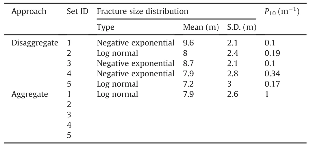
Table 2 Comparison of fracture length distribution between aggregate and disaggregate approaches.

This paper adopts a particle size distribution(PSD)approach to obtain the cumulative percentage by volume(similar to soil mechanics PSD analysis).Specific passing sizes are refereed to as P#,where the symbol P stands for passing and the symbol#represents the percentage value;for example,P50 would be the block size at 50%passing.Fig.4 shows the PSD curves for both aggregate and disaggregate approaches,and a selected visual example of the rock blocks formed on the simulated slope.Fewer but larger blocks are formed along the slope when using an aggregate approach.The P50 passing for the aggregate approach is 0.8 m3,compared to 0.6 m3for the disaggregate approach;the total numbers of blocks generated are 594 and 1118 for aggregate and disaggregate approaches,respectively.Notwithstanding the limitation of being a relatively small dataset,the analysis shows the limitations of assigning average properties(intensity and size)to all mapped orientation data.The impact is twofold:

Fig.3.Stereonet of mapped orientation data and interpreted fracture sets(modified from King,2017,personal communication).

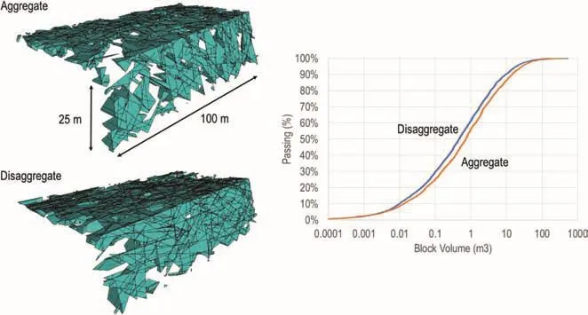
Fig.4.PSD curves for both aggregate and disaggregate approaches,and selected visual example of the rock blocks formed on the simulated slope.

(i)39%of all mapped data have an average fracture size greater than 7.9 m(value used in the aggregate DFN model).More importantly,averaging fracture size somehow diminishes the role of Set 3,which together with Set 4 contributes to most of the critical intersections forming possible blocks.When using an aggregate approach,engineers should also consider the impact that combining all data in one single set may have in terms of fracture intensity.

(ii)Since theP10conditioning technique(with fractures being generated until the targetP10is reached)would be applied using all orientation data,the set(or sets)whose dip/dip direction with respect to the scanline trend/plunge is such that it minimises the orientation bias would likely be oversampled in the overall fracture network.As shown in Table 3,Sets 1 and 3 are under-sampled since the overall target intensity of 1 m-1is reached before a sufficient number of fractures belonging to those sets are generated,while Set 5 is over-sampled.However,orientation biases are accounted for when using aP10conditioning technique in combination with a disaggregate approach,since each set is generated independently using specificP10targets.

3.2.Field mapping and DFN modelling of a large-scale slope

The results of the preliminary DFN analysis indicated that the approach used in generating a DFN model can have a significant influence on the simulated IBSD.To further investigate the topic,the study was expanded to include data collected for a larger(unnamed)slope.The orientation,length,and location(geo-referenced)of more than one thousand fractures were measured as partof an extensive field mapping campaign.The data collection and processing for DFN analysis were documented in Schlotfeldt et al.(2018).The abundance of deterministic data makes the dataset ideal for studying the differences between conditioned and unconditioned DFN models.

Table 3 Comparison of P10intensity between aggregate(simulated P10)and disaggregate(target P10)approaches.

The objectives of the second case study include:

(i)Investigation of the influence of aggregate vs.disaggregate approach on rock block analysis results with respect to the fracture sets’orientations and lengths;and

(ii)Generation of a conditioned DFN model to assess the influence of deterministic fractures on simulated IBSD.

3.2.1.DFN model generation

Three DFN models were considered in the current study:Model 1,fully stochastic DFN model using disaggregate approach;Model 2,fully stochastic DFN model using aggregate approach;and Model 3,conditioned DFN model using disaggregate approach.Field mapping was carried out as a combination of several vertical scanlines(rope access)and areal mapping(photogrammetry).The latter was the sources for fractures length data.The input parameters used for the DFN model generation are summarised in Table 4.All five fracture sets(J0 to J4,Fig.5)follow similar fracture length distribution except J0,which is the most abundant mapped fracture set.In contrast,most of the fractures in J1,J3 and J4 were not mapped in the field;therefore,few deterministic fractures are incorporated into the conditioned DFN model for those fracture sets.The volumetric intensityP32is approximately the same for all fracture sets except J3.For generating the conditioned DFN models that included deterministic fractures,a procedurehad to be devised to reassess the intensity of the stochastic fractures to balance the overall fracture intensity for the model.The 4-stage process includes:

(i)Generation of stochastic fractures within a box with volumetric intensity(P32S)determined from the mapped data;

(ii)Import of the deterministic fractures into the model and measure the volumetric intensity of those fractures(P32D);

(iii)Removal of all stochastic fractures;and

(iv)Re-generation of stochastic fractures using a new volumetric intensity adjusted to account for the contribution of the deterministic fractures(P32S-P32D)and removal of large stochastic fractures yielding larger traces that would not correspond to field observations.

Table 4 Input parameters for the DFN models.

Fig.5.Stereo plots of fracture orientation.Mapped data(left)and simulated data using a disaggregate approach(right).

Note that a required input parameter to generate a conditioned DFN model is the tracemap corresponding to the mapped fracture traces.Manual window and scanline mapping techniques in addition to photographs can be used to sketch a simplified tracemap.However,for the slope under consideration,this type of information was more objectively captured using remote sensing techniques(photogrammetry)to better geolocate deterministic fractures.

3.2.2.Block size analysis

Five realisations were generated for each model type,and examples are shown in Fig.6,in which the red coloured fractures for Model 3 represent the deterministic fractures.Other colour differences in Fig.6 for Models 1 and 3 represent different stochastic fractures sets.The rock block analysis is performed for both the north and south walls.

Figs.7-9 present the IBSD for Models 1-3(south and north walls),and the curves represent 5 different DFN realisations(a-e).For each model type,the results of the 5 DFN realisations were then combined into an average size distribution curve(Fig.10).The results show that for Model 3,there are no major differences when selecting either the south or the north wall as a sampling plane,since it mostly includes deterministic fractures belonging to Set J0,which occur on both sides of the narrow slope region.However,Model 2 shows a significant difference between the size of the blocks generated on the south and north walls.The difference could be explained by considering the smaller size distribution parameters(Table 2)that are assigned to J0 when using an aggregate modelling approach(3 m and 7 m average fracture lengths for aggregate and disaggregate models, respectively). When comparing Models 1 and 3(disaggregate),the results show the role that the deterministic fractures play in IBSD;the P50 passing sizes are 0.096 m3and 0.073 m3for Models 1 and 3,respectively.

When considering the tracemaps generated by the stochastic and deterministic fractures on the south wall,Model 3 yields the lowest areal intensity(P21)at 1.4 m-1.Models 1 and 2 yield areal intensity values of 1.57 m-1and 1.62 m-1,respectively(Table 5 and Figs.11-13).Field estimates ofP21for an equivalent slope region as the one simulated in the current models were in the range of 1.2-1.5 m-1(Elmo,2018,personal communication).Clearly,disaggregate models and models that include deterministic fractures would guarantee a better agreement with field conditions,compared to models that aggregate fractures into one homogeneous set.In terms of spatial location,in Model 1,the fractures belonging to Set 0 are more evenly distributed in space compared to those in Model 3,in which the location of the J0 fractures is imposed by the deterministic nature of the model.This would have clear implications with respect to design scenarios since block location would reflect the concentrations of 2D traces on the sampling plane or slope.But concentrations of 2D traces forming closed polygons would not necessarily imply that a 3D block exists,as discussed in more details in Section 4.3.

Fig.6.Selected examples of DFN Model 1(disaggregate approach),Model 2(aggregate approach)and Model 3(conditioned model and disaggregate approach).

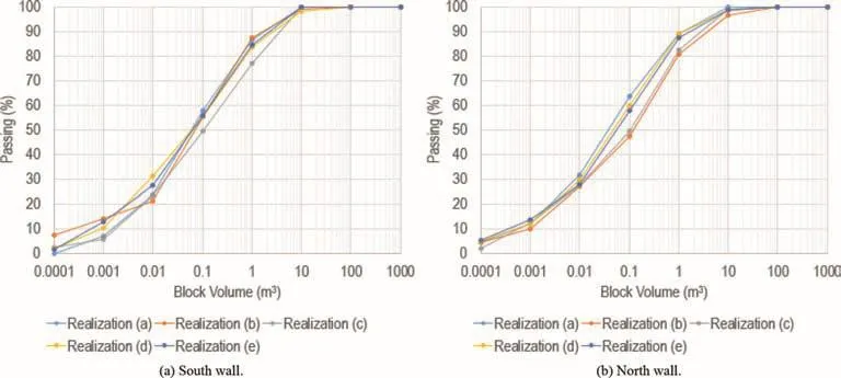
Fig.7.Comparison between the PSD for Model 1,south and north walls.

Fig.8.Comparison between the PSD for Model 2,south and north walls.

The results show another instance of variability that is ultimately a function of the randomness of geological processes,whereby for a fully stochastic analysis(e.g.Models 1 and2),the spatial locations of blocks and their sizes would vary,depending on which DFN realisation is considered.In contrast,less variation is observed for the conditioned model(Model 3),in which the occurrence of georeferenced deterministic fractures controls the formation of blocks in the left side and lower part of the south wall.Similarly,Model 3 shows a consistency in terms of shape and number of blocks,independent of which DFN realisation is considered.

3.3.Anisotropic effect of discontinuity sets on kinematic stability analysis

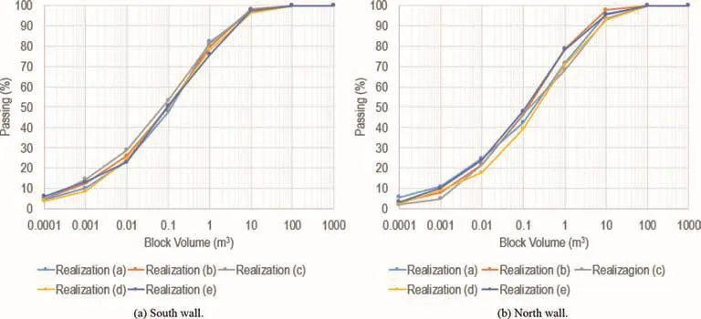
Fig.9.Comparison between the PSD for Model 3,south and north walls.

Fig.10.Comparison between the PSD for Models 1-3,south and north walls.

Table 5 Comparison of P21(m-1)between the models,south and north walls.

Fig.11.Model 1;tracemaps for DFN realisation(a)and outlines of blocks formed on south wall for DFN realisation(a-c).

Fig.12.Model 2;tracemaps for DFN realisation(a)and outlines of blocks formed on south wall for DFN realisation(a-c).

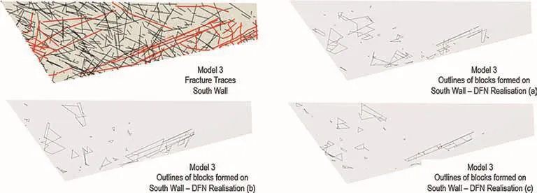
Fig.13.Model 3;tracemaps for DFN realisation(a)and outlines of blocks formed on south wall for DFN realisation(a-c).Thick red lines represent deterministic tracemaps.

The randomness of natural geological processes raises the important question:Whether it is reasonable to make design decisions based on a single calculated factor of safety,or considering a risk assessment approach.The results of the DFN analysis presented in Sections 3.1 and 3.2 demonstrate that DFN models can better capture the variability of the parameters used for kinematic stability analysis.There are important aspects that geotechnical engineers should consider when using a stochastic DFN approach to design:

(i)An objective field mapping approach is required to guarantee that data variability is effectively captured in DFN models(Elmo et al.,2016).In this context,data variability can be defined as the observable manifestation of heterogeneity of physical parameters,and should not be confused with data uncertainty,which reflects the decision to describe the observed variability in a qualitative or quantitative manner.

(ii)With respect to field mapping of natural fractures,fracture length is an important parameter for DFN modelling,as demonstrated when generating a DFN model using either an aggregate or disaggregate approach.However,either fracture length is seldom available due to the lack of exposures,or engineers have access to limited length data collected along exploratory drifts.Mapping of fracture length should also consider both trace length bias and the effects of cut-off assumptions that are inherent in any mapping methodology.

(iii)Remote sensing techniques should be used whenever possible to integrate the data collected using more conventional methods(e.g.core logging and manual mapping of surface exposures).Deterministic data should then be integrated with stochastic models to generate so-called conditioned DFN models.Whereas the results would still need to be interpreted in the context of probability of failure,the analysis would better reflect the spatial location of potential unstable blocks.

In the authors’opinion,the aspects above represent the driving theme that could force engineers to think about the importance of uncertainty and variability in rock engineering design and embrace new methods of data collection and analysis.

4.Quantification of GSI using a DFN approach

Since the 1970s,with the increasing use of numerical modelling for rock engineering design,researchers have discussed the need of estimating rock mass properties from intact properties and discontinuity properties.The Hoek-Brown failure criterion(Hoek and Brown,1980;Hoek et al.,2002)was indeed developed to address the need of establishing representative rock mass properties as a function of the intact rock strength,rock type,degree of fracturing and joint conditions.The Hoek-Brown criterion requires the knowledge of GSI to define the rock mass quality.Since its conception(Hoek et al.,1995),GSI represented a true qualitative assessment of rock mass quality,with no specific ratings assigned to determine joint condition and blockiness of the rock mass.

Although the GSI system has been proven to be useful when used by experienced engineers,they may find estimating the GSI values a difficult task due to the lack of measurable references.For those reasons,several attempts have been made in the literature to“quantify”GSI,including:

(i)Sonmez and Ulusay(1999)proposed a quantification of GSI using structure rating(SR)and surface condition rating(SCR).SCR is the sum of ratings for roughness,weathering,and infilling.To represent the blockiness of the rock masses,the authors suggested using a rating(SR)that could be obtained from the volumetric joint count(Jv),which is a measure of the degree of jointing or the inter-block size(Palmstrom,2005).

(ii)Cai et al.(2004)proposed a quantification of GSI using joint condition factorand block volume as measurable ratings.The joint condition factor was adopted from the RMi classification system proposed by Palmstrom(1995).

(iii)Russo(2007,2009)recognised that a correlation could be established between GSI and the joint parameter(JP)in RMi system,using the constantssandain the Hoek-Brown failure criterion.

(iv)Hoek et al.(2013)proposed a quantification of GSI using the rock quality designation(RQD)to represent the blockiness of the rock masses,and the joint condition rating from the 1989 version of the rock mass rating(Bieniawski,1989).

One of the challenges that engineers face when estimating GSI concerns the fact that field observations are limited to either 1D or 2D exposures(e.g.boreholes logs,slope faces and tunnel walls),when truly the degree of rock mass blockiness and interlocking is a 3D parameter(Fig.14).Fractures forming an enclosed polygon in 2D space may not necessarily form a block in 3D space;therefore,actual 3D rock mass fragmentation may be significantly different from the one inferred from 2D observations.In this paper,the authors use the DFN models to compare the 3D rock block forming potential with the 2D connectivity of fractures on a plane.

Using data collected at a room-and-pillar mine,this section is dedicated to the study of a new approach to provide a quantitative assessment of GSI,with the objective to facilitate establishing possible ranges of GSI for a given rock mass domain.The approach integrates the method proposed by Cai et al.(2004)with DFN analysis of IBSD.The authors believe that the proposed method could provide a better and more objective quantification of GSI variability.

Note that the GSI ratings’table is based on the underlying assumption that the rock mass is isotropic and homogeneous.However,the GSI can still be applied(with caution)to anisotropic rock masses if the failure of such rock masses is not controlled by structurally controlled failure(Marinos et al.,2005).To further examine the validity of such a statement,this study considers both the case of an isotropic rock mass and a transversely anisotropic rock mass that includes bedding features.

4.1.DFN model generation

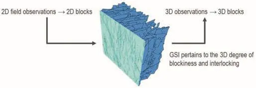
Fig.14.Estimating a 3D rock mass classification rating requires access to 3D information.

The analysis is performed using data collected by the second author at a classic square room-and-pillar mining operation in Derbyshire,UK(Elmo,2006).Details about the data collection process and field observations were presented in Elmo(2006).A new DFN model was generated and improved based on the one included in Elmo(2006).It should be noted that for this specific site,the quality of the field data was not typical of many engineering projects.The second author personally supervised the data collection process and the data were collected using new guidelines designed to address some of the limitations of the ISRM(1981)suggested methods for quantitative description of discontinuities in rock masses in relation to DFN theory and principles.Through data characterisation process,it was possible to identify 3 main fracture sets(Sets 1-3,Fig.15).Set 1 strikes roughly NE-SW and Set 2 NW-SE.Set 3 is a more widely spaced set striking W-E and dipping at about 45°to both North and South(bivariate distribution).In addition,there are widely spaced,near horizontal bedding planes.Based on the analysis of mapped trace lengths,Set 1 was divided into two subsets.Set 1a includes relatively long fractures that extend over the full height of the pillars,while Set 1b mostly includes shorter fractures(maximum 5 m).Sets 2 and 3 were also divided into subsets(2a and 2b;3a and 3b)based solely on orientation data to facilitate model generation.Except for Sets 1a,3a and 3b,differences in terms of mapped fracture size and fracture frequency are not significant.This is an important aspect to be considered when later discussing differences that may exist between outputs(i.e.block size)generated based on the simulated fracture networks.

The analysis considered generating the DFN models using both an aggregate and a disaggregate approach.In the former,no difference is made between the sets,and a single distribution for fracture intensity and fracture size is applied to all sets(1,2 and 3).In the latter,each fracture set is treated separately,and all sets are then combined to obtain the overall representation of the fracture network.Furthermore,two types of DFN models were considered,based on whether they included only stochastic fractures(joints,Sets 1-3),or stochastic fractures(joints,Sets 1-3)in addition to bedding features treated deterministically.The complete list of DFN models included:

(i)Model 1:DFN model without bedding planes generated using aggregate approach.

(ii)Model 2:DFN model with bedding planes generated using aggregate approach.

(iii)Model 3:DFN model without bedding planes generated using disaggregate approach.

Fig.15.Stereonet of mapped orientation data and interpreted fracture sets for the Middleton mine dataset.Bedding data are not included.Bedding was observed to be very low dipping(horizontal).

(iv)Model 4:DFN model with bedding planes generated using disaggregate approach.

A disaggregate approach requires the determination of statistical distributions for each fracture set.The volumetric intensity(P32)of each fracture set is determined from the correlation with the linear intensity(P10).Bedding planes were modelled assuming an average spacing of 3 m,imposed using aP10conditioning method,whereby bedding planes are generated in the model such that the average spacing is approximately 3 m,and the bedding planes may be generated anywhere across the full height of the pillar.The equivalent radius distribution is assumed to be equivalent to the trace length distribution obtained from the mapped length of fractures.The properties used in the generation of the DFN models are presented in Table 6.Examples of DFN models are shown in Fig.16.

4.2.Rock block analysis and characterisation of GSI variability

Five realisations are generated for each of the 4 types of DFN models.Once the models are generated,a rock block analysis tool is used to define potential block forming when intersecting a series of sampling planes oriented vertically and horizontally(Fig.17).

When considering the horizontal sampling planes(Surfaces 5,6 and 7),the block search analysis is performed with respect to the top side of the surface,while for Surfaces 1,3 and 4,the block search analysis is performed such that the blocks would be contained inside the pillar region.PSD curves(block volume)are then compared using both P20 and P80 percent passing as the key indicators of finer and coarser sizes,respectively.Because of the stochastic nature of DFN modelling,multiple realisations are considered in the analysis.Additionally,tracemaps generated for Surfaces 1,2 and 3 are used to study the difference between apparent 2D rock mass fragmentation(fracture traces forming closed polygons)and the actual fragmentation associated with the creation of 3D blocks.

Fig.18 shows the PSD plots for DFN Models 1-4.The curves represent the average block volume for all vertical surfaces combined(Surfaces 1,2,3 and 4)and all horizontal sampling planes combined(Surfaces 5,6 and 7).Figs.19-22 show the variations of block volume for each model for one of the realisations.The PSD plots are separated with respect to vertical and horizontal samplingplanes since the results for the latter are strongly influenced by the location of the bedding features.

Table 6 Properties used to generate the 4 different DFN models.

Fig.16.Examples of generated DFN models.From left to right:Model 1(aggregate),Model 2(aggregate with bedding features),Model 3(disaggregate),and Model 4(disaggregate with bedding features).

Fig.17.Location of the sampling planes used in the rock block analysis.

Fig.18.PSD plots of block volume for Models 1-4.All vertical and horizontal sampling planes are combined.

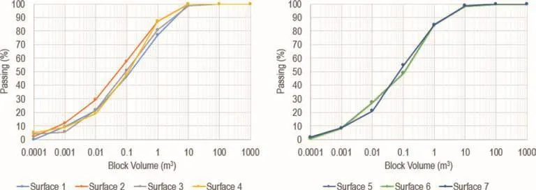
Fig.19.PSD plots of block volume for Model 1(aggregate,no bedding),vertical(Surfaces 1-4)and horizontal(Surfaces 5-7)sampling planes.

Fig.20.PSD plots of block volume for Model 2(aggregate,with bedding),vertical(Surfaces 1-4)and horizontal(Surfaces 5-7)sampling planes.

Fig.21.PSD plots of block volume for Model 3(disaggregate,no bedding),vertical(Surfaces 1-4)and horizontal(Surfaces 5-7)sampling planes.

Fig.22.PSD plots of block volume for Model 4(disaggregate,with bedding),vertical(Surfaces 1-4)and horizontal(Surfaces 5-7)sampling planes.

The results clearly show that block forming potential depends on the modelling assumptions(aggregate vs.disaggregate),and on whether vertical or horizontal free surfaces are used as sampling planes.There is no major difference between block volumes generated along Surfaces 1-4 for aggregate DFN models(e.g.Fig.20),but disaggregate models with bedding features(Fig.22)yield relatively smaller block sizes compared to aggregate models(Fig.20).Bedding features have a strong impact on block forming potential,as a function of the relative location of the sampling plane and the bedding features(e.g.Fig.19 vs.Fig.20;and Fig.21 vs.Fig.22).Because of the stochastic nature of the models,block forming potential(and block size)would depend on the relative location of the fractures with respect to the sampling planes.This has clear implications for determination of the IBSD,since it would be a function of the orientation and location of the mapping surface(Fig.23).

Using the quantification of GSI proposed by Cai et al.(2004),the block volumes corresponding to the P20 and P80 passing sizes in the PSD curves define the minimum and maximum ranges of IBSD for the simulated rock mass,respectively.Mapping data(Elmo,2006)showed that joints were smooth to rough(average joint roughness coefficient(JRC)of 10)and slightly weathered,which in the GSI system would correspond to good jointing conditions.By combining the range of blockiness with jointing conditions(Table 7and Fig.24),it is possible to define a range of GSI ratings for Models 1-4.In addition to P20(lower bound)and P80(upper bound),smaller ranges of GSI corresponding to P30-P70 passing sizes and single GSI corresponding to the P50 passing size are also included in the results.

Table 7 Comparison of GSI ranges corresponding to P20-P80,P30-P70 and P50 size passing.

Because of its definition(disaggregate approach with bedding features),Model 4 would be the one that more realistically simulates the fracture network for the mapped pillars(vertical exposures)at Middleton mine.According to field observations(Pine and Harrison,2003;Elmo,2006),the GSI for the pillars at Middleton mine was in the range of 60-70.Note that those field estimates would be based on a qualitative assessment of rock mass blockiness and may be biased towards the larger block size due to the inherent propensity of a person that collects data in the field to focus on the largest visible structures.Overall,the quantitative measurements of GSI ratings for both Models 4 and 2 are in good agreement with field observations.Model 3 is the one that least resembles field conditions,and in fact largely underestimates the rock mass quality.The results therefore show the importance of creating DFN models taking into consideration differences that may exist between fracture sets.The quality of the input data likely contributed to reducing model uncertainty,thus it would further explain why generally only minor differences were observed in some of the DFN models in terms of estimated block size.

Fig.23.Comparison of blocks being formed on Surfaces 1-4 for Model 2(top row)and Model 4(bottom row).

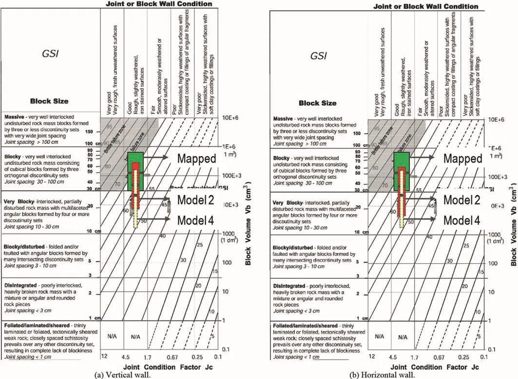
Fig.24.Comparison of variation of GSI ranges for the 4 DFN models generated for Middleton mine.Green dot represents P50,the thick orange line and the thin black line represent the P30-P70 and P20-P80 size passing ranges,respectively.Results for Models 2 and 4 are given with respect to the modified GSI charts by Cai et al.(2004).

To further test the approach,the results for the large-scale problem presented in Section 3.2(south wall)were also analysed in terms of rock mass blockiness(Table 8 and Fig.25).Jointing conditions were characterised as fair to good based on field mapping data.The results highlight the relative importance of both the quality of data collection and the need of generating DFN models that reflect the structural geology of the site,since in this case Model 2(aggregate model,no deterministic fractures)would overestimate the rock mass quality compared to Models 1 and 3.

4.3.Limitations of 2D surveys to determine rock mass blockiness

The estimation of a GSI rating for a rock mass is commonly based on 1D(boreholes)and 2D(surface outcrops) field data.1D data areintrinsically limited as they cannot provide a measure of fracture length,and the authors argue that alternative 1D indicators such as RQD(Deere et al.,1967)cannot provide a quantitative assessment of rock mass blockiness because of the sensitivity of RQD measurements in terms of orientation bias and minimum length below which core pieces are not included in the calculation.Likewise 2D data are also affected by orientation bias,and fully formed blocks may be perceived based on whether intersecting fracture traces form closed polygons.Figs.11-13 in Section 3.2 provided an initial example of the difference between the location of fully formed 3D blocks in relation to 2D tracemaps.

Table 8 Comparison of GSI ranges corresponding to P20-P80,P30-P70 and P50 size passing for the slope model described in Section 3.2(south wall).

Fig.25.Variation of estimated GSI for the large-scale slope problem discussed in Section 3.2(south wall).

Fig.26.Comparison between 2D perceived blocks and actual 3D blocks formed across Surfaces 1-4(see Figs.17 and 23)for Model 2(top)and Model 4(bottom).

Using the DFN model developed for Middletown mine(Type 2,aggregate approach with bedding features;and Type 4,disaggregate approach with bedding features,respectively),Fig.26 shows the tracemap generated on Surface 1 for one DFN realisation,and the 3D blocks formed by the intersection of the DFN model with Surfaces 1-4.It is possible to identify the largest 2D polygonal areas on the tracemap and compare it with the area corresponding to 3D blocks.Note that a direct comparison would only be possible using data for Surface 1;tracemaps for Surfaces 2-4 were not included to minimise the number of figures in the manuscript;however,Fig.26 still provides a qualitative comparison between the different sampling planes used in the analysis.

The difference between the enclosed 2D areas and the actual area corresponding to the 3D blocks intersection areas is relatively small for Model 2-Surface 1,but relatively large for Model 4-Surface 1,due to the difference assumption made with respect to fracture size in the aggregate and disaggregate models when generating the stochastic fractures.The perceived blockiness observed on a 2D plane does not necessarily correspond to the true 3D blockiness of the rock mass;therefore,estimates of GSI based on perceived 2D blockiness may yield overly either conservative or nonconservative ratings for smaller and larger 2D blocks,respectively.Likewise,there could be a high variation in block forming potential depending on the location of the sampling plane.In this context,DFN models offer the opportunity to characterise this variability and provide better estimates of rock mass blockiness.

5.Conclusions

This paper describes different applications of DFN modelling to characterising block stability and rock mass blockiness for naturally fractured rock masses.Two aspects of data characterisation process are examined in the first part of the paper:(i)influence of generating a DFN model using either an aggregate or a disaggregate approach;and(ii)influence of incorporation of deterministic fractures into the DFN model.Key observations included:

(1)The selection of aggregate vs.disaggregate approach could have a significant influence on kinematic stability analysis.Using an aggregate approach,important input parameters such as fracture intensity and fracture size could be either overestimated or underestimated.Accordingly,both the size and the number of unstable blocks may not be truly representative of field conditions.

(2)A conditioned DFN model that includes major deterministic fractures would allow for a better consideration of the spatial location of potentially unstable blocks.

The second part of the paper addresses the fundamental questions related to the estimation of GSI from rock block analysis using DFN models.Three key aspects have been examined:(i)estimation of GSI ratings for rock masses that contain well defined bedding features;(ii)determination of GSI ratings to better reflect the variability of rock mass blockiness;and(iii)implication of using 2D vs.3D data to characterise rock mass blockiness.The results showed that the variation of GSI could be as large as±12.This has clear implications for design scenario since it shows the limitations of using a single point estimate of GSI to establish rock mass behaviour.

Furthermore,we believe that these results offer anew perspective on rock mass classification systems.Because of the inherent variability of the underlying rock mass fabric,classification ratings are not supposed to provide exact measurements of rock mass quality.In the original version of the GSI system,Hoek et al.(1995)included a comment warning engineers and practitioners not to seek precision,but rather to use a range of GSI values.Despite that,many engineers and practitioners still perceive rock mass ratings as intrinsic rock mass properties,to the point,for example,of mistakenly stating GSI ratings with decimal precision.The results of the analysis show that the variability of rock quality may be such that an acceptable GSI range may be obtained even when using data that contain a certain degree of uncertainty(i.e.Model 2 in Fig.24).The following conclusions could be drawn:(i)the issue of putting numbers to geology retains its challenge and engineers need to accept that rock masses are spatially variable,and their quality cannot be described by a single rating;and(ii)classification methods may need to be developed that are more sensitive to data uncertainty,by using a unique set of rock mass properties directly instead of assigning a rating based on the value of a measured rock mass property(e.g.measurements of fracture frequency and fracture spacing).

As more general remarks,this paper has further demonstrated that a DFN approach can take full advantage of fracture data collected from mapping of exposed surfaces and boreholes,including also digital photogrammetry and laser scanning techniques.Despite these advantages and the range of applications that DFN models offer to engineers,including those discussed in this paper,many still regard the subject of DFN modelling with doubt and suspicion.There may be practical reasons that limit the applications of DFN modelling(e.g.lack of adequate data to generate a realistic and useful model),but other reasons may be as simple as the difficulty to understand the concepts(and the language)behind the DFN approach.Notwithstanding,the authors believe that DFN modelling could be used as a toolbox to bring the fundamental concepts of statistics,structural geology,data collection and rock mass characterisation together,offering a path to better account for uncertainty and variability in rock engineering design.

Conflicts of interest

The authors wish to confirm that there are no known conflicts of interest associated with this publication and there has been no significant financial support for this work that could have influenced its outcome.

Acknowledgments

The authors would also like to thank NSERC(Natural Sciences and Engineering Research Council of Canada)for the financial support provided to this research through a Collaborative Research Development grant(Grant No.11R74149;Mine-to-Mill Integration for Block Cave Mines).We would like to express our gratitude to Golder Associates Ltd.for providing an academic license for the code FracMan.This paper was originally presented at the 15th IACMAG Conference(Wuhan,China,19-23 October 2017)and has subsequently been revised and significantly extended before consideration by theJournal of Rock Mechanics and Geotechnical Engineering.