Simulating hydraulic fracturing processes in laboratory-scale geological media using three-dimensional TOUGH-RBSN

Disuke Ashin,Pengzhi Pn,Kimikzu Tsusk,Mikio Tke,John E.Bolner

aGeological Survey of Japan,Ibaraki,Japan

bState Key Laboratory of Geomechanics and Geotechnical Engineering,Institute of Rock and Soil Mechanics,Chinese Academy of Sciences,Wuhan,430071,China

cINPEX Corporation,Tokyo,Japan

dUniversity of California,Davis,USA

Keywords:Hydraulic fracture Crack opening TOUGH Rigid-body-spring network(RBSN)Permeability Injection pressure Fluid viscosity Hydro-mechanical(HM)processes

A B S T R A C T

1.Introduction

Hydraulic fracturing techniques in geological engineering typically involve interactions between hydraulic and mechanical processes.Elevated fluid pressure creates fracture formation in geological media,which induces significant changes in permeability.Proper operations of the hydraulic fracturing are important for optimizing hydrocarbon extraction and enhancing geothermal systems,as well as minimizing environmental impacts related to the contamination of freshwater resources (Valko and Economides,1996;McGarr et al.,2002;Rubinstein and Mahani,2015).However,the permeability evolution of geological media can be difficult to be predicted,because it depends on not only the appearance of the hydraulic fractures,but also the interactions with pre-existing natural fractures and various geological conditions.

Various analytical solutions to the hydraulic fracturing problem have been proposed,and they have facilitated understanding of the importance of hydro-mechanical(HM)interactions(Perkins and Kern,1961;Geertsma and de Klerk,1969;Nordgren,1972;Detournay,2004;Adachi et al.,2007).However,they generally suffer from the limitations associated with simple fracture geometries,which exclude evolutionary problems in domains with real complexity.Researchers have also conducted field experiments and analog laboratory studies on hydraulic fracturing behavior (Legarth et al.,2005;Guglielmi et al.,2015).Physical testing is an effective means for studying various aspects of hydraulic fracturing,but such testing is limited by(i)the expense of conducting parametric studies,and (ii)difficulties in reproducing the anticipated environmental conditions.Numerical modeling is less constrained by these factors,and can therefore serve as a complimentary investigation technique.

Many of the advances in modeling hydraulic fracturing processes have been accomplished within the framework of finite element techniques,based on a continuum modeling of fracture and damage(Boone and Ingraffea,1990;Secchi and Schrefler,2012;Settgast et al.,2017).The hydraulic fracturing of heterogeneous rock samples has been modeled by a three-dimensional(3D) finite element method(FEM)that accounts for the coupled HM processes(Li et al.,2012).Recent developments in the extended FEM have also been used to simulate strong discontinuity in displacement during hydraulic fracturing(Irzal et al.,2013;Mohammadnejad and Khoei,2013).

To model multiple fractures or fracture networks,discrete element and/or particle methods have been developed for analyzing hydraulic fracturing processes under a variety of geological conditions.Discrete element methods have been used to study HM interactions in fluid-induced fracturing processes,and their collective influence on the behavior of geological systems.The effect of injected- fluid pressure on fault reactivation or well bore has been studied for micro-seismicity impacts using two dimensional(2D)discrete element methods(Shimizu et al.,2011;Yoon et al.,2015).Lattice-type approaches are another means for studying HM interactions in fluid-induced fracturing processes for a variety of geomaterials(Tzschichholz and Herrmann,1995;Flekkøy et al.,2002).Dual-lattice models,linkages between cracks within the structural lattice,and their transport properties within the flow lattice,are developed to model concrete deterioration,by simulating dynamic flows during fracture development(Nakamura et al.,2006;Saka,2012;Grassl et al.,2015;Grassl and Bolander,2016).Kim et al.(2017)used a lattice model based on the rigid-body-spring network(RBSN)coupled with a multiphase fluid flow simulator,TOUGH2(Pruess et al.,1999),to conduct planar analyses of hydraulic fracturing in a rock-analog sample,which contained designed pre-existing fractures.Various alternative approaches are also available,such as the use of cellular automata(Pan et al.,2013,2014),or boundary element methods(Sousa et al.,1993)to simulate hydraulic fracture processes in geomaterials.

Although effective mechanical-damage models are available in the literature,their ability to simulate coupled HM processes remains limited,especially when they are used to model fracture propagation in 3D(Settgast et al.,2017).The 3D models are needed to study the mechanisms of hydraulic fracturing processes,and their results must be compared with controlled and reliable data sets(e.g.laboratory tests).Validated computer models offer a controlled environment to study the stochastic nature of geological media.

In this paper,we further present the development of an existing 3D HM simulation tool to model hydraulic fracturing processes in geological media at laboratory scale.The first part of the paper summarizes the recent work on the coupled HM simulation tool,TOUGH-RBSN(Asahina et al.,2014).TOUGH2 is used to simulate flow and transport through discrete fractures and within porous rocks(Pruess et al.,1999),whereas elasticity and fracture development are simulated by a lattice model based on the RBSN concept(Kawai,1978).Herein, the approach is extended for 3D analyses of hydraulic fracturing experiments with special attention to stress and damage-induced hydraulic properties.The capabilities of the modeling approach are demonstrated through(i)transient pulse tests performed during triaxial compression loading on Shirahama sandstone,and(ii)analyses of static fracturing due to fluid pressure.Thereafter,the model is used to simulate laboratory tests of hydraulic fracturing in granite samples,to evaluate how fluid viscosity affects the hydraulic fracturing processes.The fracture events and their patterns during a progressive failure process are also discussed.It is possible to activate dynamically flow pathways that form along a discrete fracture,in which fracture nodes and their associated connections are introduced at the Voronoicell boundary.

2.Methodology

This section presents a background description of the existing codes:TOUGH2,a multiphase flow and transport simulator developed at the Lawrence Berkeley National Laboratory(Pruess et al.,1999),and RBSN,which is used to model the elasticity and fracture development of geomaterials(Bolander and Saito,1998).The linkage of TOUGH2 to RSBN is also briefly described in this section.Additional model details can be found in the literature(Asahina et al.,2014;Kim et al.,2017).

2.1.Hydrological modeling:TOUGH2 simulator

TOUGH2 is a widely used general-purpose numerical code for simulating the non-isothermal flow of multiphase,multicomponent fluids in permeable media.The integral finite difference method is used as the numerical solution scheme,and is compatible with both structured and unstructured numerical grids.The simulations presented here use TOUGH2 with Module 1 equations of state,which account for water present in liquid,vapor,and two phase.Literature related to the TOUGH2 simulator can be found elsewhere(Pruess et al.,1999;Cappa and Rutqvist,2011;Pan et al.,2014).In a previous study,the authors developed an approach within TOUGH2 for representing discrete fractures in a permeable porous medium,in which the computational domain was effectively discretized as the Voronoi tessellation of a spatially random set of points(Asahina et al.,2014).

In this study,we modified the original TOUGH2 grid structure to accommodate the formation of flow associated with fracturing.As shown in Fig.1a and b,an interface node is newly inserted at the Voronoi cell boundary.To activate flow pathways between matrix and interface nodes,new sets of connections(matrix-interface connections)are introduced between associated nodes.The original matrix-matrix connection is divided into two matrix-interface connections.In addition,the neighboring interface nodes are connected,to activate flow pathways in the discrete fracture,which are generally assumed to follow Darcy’s law.The hydraulic properties of discrete fractures,such as permeability and porosity,can be assigned by either grid geometry or fracture apertures,which are computed by the mechanical models described below.

2.2.Mechanical-damage model:RBSN

We modeled the elasticity and fracturing of geological media using a RBSN,a special type of lattice model(Kawai,1978;Bolander and Saito,1998;Asahina et al.,2017).The model formulation is briefly described in this section.The positions of the nodal points are determined by Voronoi nuclei,and the topology of the RBSN is defined by the dual Delaunay tessellation,as shown in Fig.1c.Lattice elementijis constructed by rigidly connecting the paired pointsiandjwith a zero-size spring set.For 3D modeling,the spring set is composed of three axial springs and three rotational springs, with a stiffness matrix D= （1 ω）diag[kn，ks，kt，kφn，kφs，kφt?in localn-s-tcoordinates,whereωis a scalar damage parameter,in the range 0?ω?1,used to model material fracture.Prior to crack initiation,ω=0,and for complete damage as the traction free crack condition,ω=1,in correspondence with classical lattice approaches for modeling material breakdown(Herrmann and Roux,1990;Schlangen and van Mier,1992).The stiffness coefficients are assigned as follows:

Fig.1.2D description of nodes and connections in TOUGH-RBSN simulator:(a)Ordinary rock matrix nodes and connections,(b)Insertion of interface nodes and insertion/replacement of fracture connections,and(c)Lattice element defined by nodal connectivity i-j with zero-size spring set located at centroid of surface area Aij.The planar illustration is used here for simplicity.The insertion of interface nodes and connections extends naturally to 3D.

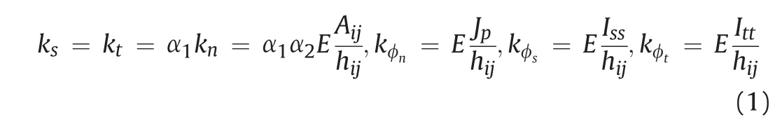
whereEis the elastic modulus;hijis the distance between nodesiandj;Aijis the area of the Voronoi boundary between nodesiandj(Fig.1c);andJp,Iss,andIttare the polar and two principal moments of inertia,respectively,of the Voronoi polygon,with respect to its area centroid.Element matrices are assembled to form system equilibrium equations in the conventional manner.Macroscopic modeling of both elastic constants(Eand Poisson’s ratio, ν)is possible by adjusting α1and α2in accordance with experimental results.For the special case ofα1= α2=1(which was used for the simulations presented herein),the RBSN is elastically homogeneous under uniform modes of straining,albeit with zero effective Poisson’s ratio(Bolander and Saito,1998).Recently,Asahina et al.(2017)developed an approach for accurately representing both elastic constants(Eandν),while retaining the simplicity and advantages associated with the use of lattice elements.Unlike conventional lattices or discrete models,the elastic constants are represented without any need for calibration.Along with elastic uniformity of the lattice,Bolander and Sukumar(2005)and Asahina et al.(2017)have shown that uniform fracture energy is consumed along the crack trajectory in accordance with the prescribed softening relation,without significant bias from the irregular geometry of the lattice.

The strength properties of a lattice element are defined by the Mohr-Coulomb criterion.The fracture surface is defined by the surface inclinationγwith respect to the normal axis,the cohesioncwith the shear axis,and the tensile strengthfn(the tension cut-off).Fractures propagate along the Voronoi cell boundaries as HM-induced stresses evolve and exceed the strength of the materials.Only one element with the maximum stress is allowed to break per iteration.The spring stiffnesses of a fracturing element are isotropically reduced by degrading the stiffness matrix D.The release of spring forces generates an imbalance between the internal and external force vectors and becomes a driving force for subsequent fracture events.Additional details about element formulations and solution procedure can be found in Yip et al.(2006).

2.3.Coupling of hydraulic and mechanical damage codes

The linkage between TOUGH2 and RBSN is described in this section.The general two-code coupling procedure is based on the earlier work of Rutqvist and Tsang(2002).However,significant modifications and extensions are made for modeling fracture propagation,as discussed in Asahina et al.(2014).Data exchanges between the two codes are relatively simple,because they share the same unstructured Voronoi grid and the same set of nodes.The capabilities of the linked TOUGH-RBSN simulator were demonstrated in previous studies through the following simulations:swelling pressure test on bentonite to study stress development and effect of gas pressure with increasing saturation,and desiccation cracking in mining waste(Asahina et al.,2014).Details of the coupling procedure can be found from those articles,but are summarized here for clarity.

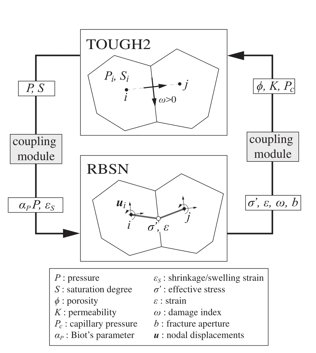
Fig.2.Flow diagram of TOUGH-RBSN linkages for coupled HM simulation.Additional nodes and connections are introduced in TOUGH2 to activate flow pathways associated with fracture(Asahina et al.,2014).

The hydraulic quantities(e.g. fluid pressure,and degree of saturation)are computed by TOUGH2,whereas the mechanical quantities(e.g.force,displacement,and damage index)are calculated by RBSN,as shown in Fig.2.External modules exchange these primary quantities between the two codes at each time step.One module supplies the fluid pressure,degree of saturation,and temperature from TOUGH2,and updates the mechanical quantities.The effective stress is calculated from the conventional Biot’s theory for porous materials(Biot and Willis,1957):

where σnis the total normal stress,is the effective stress,αPis the Biot effective stress parameter,andPis the pressure in the pores.Compressive stress and strain are positive.The incremental form of Eq.(2)can be written as

whereΔPiandΔPjare the changes in pore pressure over a time step at neighboring nodesiandj,respectively.Pore pressure only affects the mechanical element in the normal direction.It is assumed that the local changes in liquid saturation-induced strain are as follows:

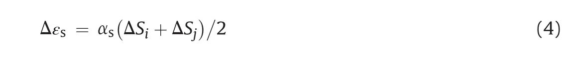
where εsis the shrinkage/swelling strain, ΔSis the change in saturation over the time step in one lattice element,andαsis the hydraulic shrinkage coefficient.ΔSis taken as the average of the two neighboring nodesiandj.For an expansive soil,the effective stress can be affected by swelling/shrinking strain as

Although the examples considered herein are limited to isothermal conditions,thermal strain can be represented by a similar formula with a thermal expansion coefficient.

After the numerical solver evaluates the deformation,another module takes the mechanical quantities from RBSN to update the hydraulic properties(i.e.porosity,and permeability)associated with the Voronoi cell and boundary in the TOUGH2 model.The hydraulic properties are functions of effective stress and strain values.In this study,except as otherwise noted,the isotropic hydraulic properties of the matrix nodes are represented by porosity mean stress and permeability-porosity relationships(Rutqvist and Tsang,2002;Pan et al.,2014).The porosityφis

where φ0is the porosity at zero-stress,φris the residual porosity,and the coefficientβ1is determined by experimental data.The mean effective stress,(in Pa),is defined as

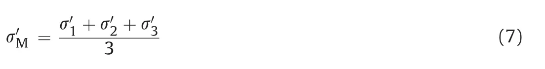
calculated at each lattice node using a method for nodal stress calculation(Yip et al.,2005).Permeability is related to porosity according to the following exponential function:

wherek0is the permeability at zero-stress,and the coefficientβ2is determined experimentally.

After a fracture is formed at elementij(i.e.ω＞0),the associated interface node is activated in the TOUGH2 model.The permeability of an individual fracture,represented by the interface node,can depend on its aperture.Herein,fracture permeability is set to a constant value to represent the experimental results.

3.Simulation of permeability evolution under triaxial compression loading

3.1.Experimental program

In this first example,we demonstrate the effectiveness of the developed coupling procedure in the 3D TOUGH-RBSN simulator.The basic framework of the experimental program partly refers to the work of Takahashi(2007),in which the permeability evolution of Shirahama sandstone samples was investigated under triaxial compression loading.Shirahama sandstone is a clay-bearing sandstone obtained from Wakayama Prefecture in central Japan.Two fluid reservoirs,8.97?105m3in volume,are placed on the top and bottom surfaces of the cored sample,with dimensions of 50 mm in diameter and 100 mm long,as shown in Fig.3.Triaxial tests were conducted with a confining pressure of 25 MPa,a pore pressure of 10 MPa,and a loading velocity of 0.05 kN/s.Permeability was measured by transient pulse tests.These were originally developed by Brace et al.(1968)at room temperature using a syringe pump,to which upstream and downstream lines were connected along the vertical axis.

3.2.Numerical simulations

3.2.1.Model description

Fig.3.Voronoi discretization of rock sample and two reservoirs(RSVR 1 and RSVR 2)for transient pulse tests in a triaxial compression test configuration.

Table 1 Summary of material properties and simulation parameters of Shirahama sandstone.

Consider the model shown in Fig.3,which represents a 3D discretization of the two reservoirs and cylinder sample(2018 nodes)subjected to triaxial compression.Table 1 summarizes the simulation parameters and physical properties of Shirahama sandstone,which are the average values obtained from three Shirahama sandstone samples.No flow is permitted across the boundaries,except at the top and bottom surfaces of the sample.For the permeability of an individual fracture,we used a constant value ofkf=1?1012m2.The permeability and porosity values for the two reservoirs are assigned as 1?1010m2and 100%,respectively.Hydrostatic pressure testing was conducted prior to triaxial loading tests.The zero-stress permeability of the sample was estimated by extending the linear assumption between permeabilities under hydrostatic and differential stress conditions.The parameters of the Mohr-Coulomb failure criterion,as shown in Table 1,are estimated from an individual series of experiments,in which 66 Shirahama sandstone samples were tested for different triaxial loading conditions(Takahashi et al.,1983).The heterogeneity of the Shirahama sandstone is represented by random cohesion assignments,which are normally distributed,with a mean value of 21.8 MPa and a standard deviation of 5 MPa.The vertical displacements of the top and bottom lattice node layers are prescribed,and constant confining stress is applied to all circumference lattice nodes in the normal,inward direction.Neither the friction of the loading plate nor the nonlinear contact conditions are considered in the model.

3.2.2.Simulation results

To partially verify the model,experimental and simulated pressures of the two reservoirs during transient pulse tests are first compared without mechanical effects,as shown in Fig.4.The reservoir pressures are also simulated by analytical methods(Hsieh et al.,1981).The degradation of differential pressure simulated by TOUGH2 generally agrees well with both the experimental data and analytical results.

Fig.5 presents the simulated differential stress(σZσX),permeability,and the number of fracture events(i.e.lattice element breakages)as a function of axial strain during triaxial compression loading.The experimental results are also shown in Fig.5a and b.Permeability is normalized by the zero-stress permeability for each test case.Stress relaxation occurred in each permeability test,because pressure pulses were applied in the transient pulse tests.

Fig.4.Time evolution of normalized differential pressure between RSVR 1 and RSVR 2 in the transient pulse test.

As shown in Fig.5a,the simulated and experimental results agree reasonably well for the initial slope of the curves.Stress gradually decreases after the highest fracture event occurs(Fig.5c).Although the material heterogeneity,assigned from a normal distribution of strength parameters,provides the residual strength to some degree,the model underestimates the post-peak toughness.Such ductile responses can be modeled by introducing a softening effect into the lattice elements(Nagai et al.,2004;Fu et al.,2017).The simulated and measured permeabilities are in general agreement,as can be seen in Fig.5b.In the early stages of the loading history,permeability decreases due to elastic contraction,while in the later stages it increases,due to the dilatancy associated with microcracks and their connections.This is also evidenced by the simulated fracture event count depicted in Fig.5c.The simulated permeability slope changes after the onset of fracture events,which occurs at approximately 75%-80%of peak stress.Simulated fracture events increase near the peak stress and in the subsequent stages.

Fig.6 shows the simulated fracture patterns of samples at different loading stages(A,B,C,and D),which are indicated in Fig.5a.In these figures,the fracturing elements are represented in darker shades.The Voronoi facets tile the breaking element and therefore the fracture surfaces.This facilitates the visualization of damage development,especially for 3D simulations.In the prepeak stage(during the loading stage between A and B),the fracture events are randomly distributed throughout the sample.In the loading stages B-C and C-D,the fractures coalesce and resemble the inclined failure pattern that is typical of triaxial compression test configurations.All of the fracture events up through the final stage are presented in Fig.6b.

4.Simulation of hydraulic fracturing test

4.1.Static fracture

The TOGUH-RBSN simulator is used to calculate the fracture development induced by pressure.The model is shown in Fig.7,which represents a discretization of a 200 mm?200 mm square sample with a unit thickness.Arrays of nodes are positioned to represent a straight line,which is horizontally arranged in the middle of the domain to stimulate a single straight fracture.The mesh size is finer in the middle and coarser in the region near the boundary.Fluid pressure is applied at the initial defect of one element in the center of the domain,as indicated by the arrow in Fig.7.A roller-type support is employed at the lattice nodes located at the top and bottom of the domain;one node is laterally restrained to avoid rigid-body motion.Fluid pressure can produce tensile stresses of sufficient magnitude to initiate cracking in the horizontal direction.

To check the calculated fracture aperture profiles,we use the theoretical solution to estimate the fracture aperture(w):

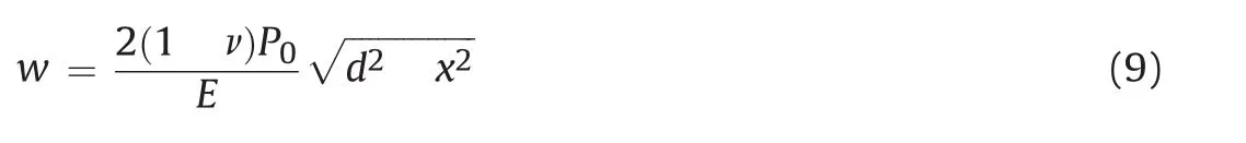
Fig.5.Triaxial compression test results as a function of axial strain:(a)Differential stress,(b)Normalized axial permeability obtained in transient pulse tests,and(c)Fracture event count within the lattice model.

whereP0is the fluid pressure within the fracture,dis the fracture width from the center,andxis the distance from the center of the fracture(Sneddon and Lowengrub,1969).Fig.8a shows the typical deformation results,and Fig.8b presents the fracture aperture calculated by the generalized displacement of the fractured lattice element for different numbers of fractured elements.The theoretical values based on Eq.(9)are also given in Fig.8b.The numerical solutions generally agree with the theoretical results.The discrepancy between the numerical and theoretical solutions grows larger with increases in the number of fractured elements.This is probably due to the boundary restraints at the top and bottom of the domain,which are not considered theoretically.Moreover,elastic deformation in the unfractured domain is not considered either.This possibly appears as discrepancy in the aperture width near the crack tip,where the numerical results are larger than the theoretical ones.In the numerical model,the unfractured elements next to the crack tip undergo tension and elastically deform.The size of discretization also affects the amount of discrepancy in the aperture width around the crack tip.

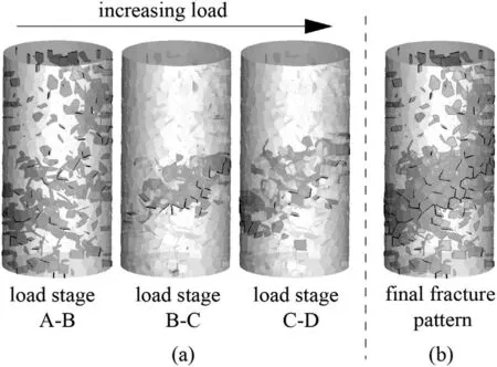
Fig.6.Simulated fracture patterns under triaxial compression loading:(a)Different load stages,and(b)Final fracture pattern.Fracturing elements appear in darker shades.

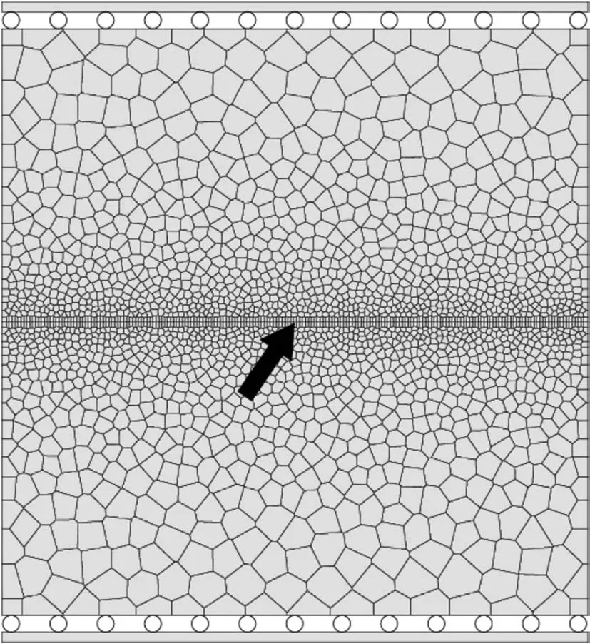
Fig.7.2D model set up for a static fracture simulation(2374 nodes).Arrow indicates the location of pressure introduction.

4.2.Rock test simulations:Hydraulic fracturing

4.2.1.Model description

Fig.8.(a)Simulated deformation results with enlarged view,and(b)Comparison between numerical and theoretical solutions for the fracture aperture from the center.n is the number of fractured elements.

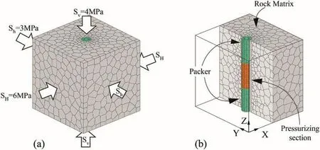
Fig.9.Domain discretization based on Voronoi tessellation of a semi-random set of points:(a)Prescribed triaxial loading,and(b)Cross-section through borehole.

In this section,TOUGH-RBSN is used to simulate hydraulic fracture processes in granite.The model parameters and model setup are taken from the experimental program of Chen et al.(2015).The 3D domain is 170 mm?170 mm?170 mm,with an injection borehole(10 mm in radius and 60 mm in length)at the center.Stiff packers are placed at the top and bottom of the borehole(Fig.9).The model is subjected to triaxial loads of 6 MPa,3 MPa,and 4 MPa in theX,Y,andZdirections,respectively.The model is discretized with 4712 nodes,corresponding to the number of Voronoi cells,and the grid size is finer around the injection hole.The territorial density of nodal points and thus the mesh discretization are controlled for reducing computational cost.Literature can be found for the treatment associated with the computational cost of large 3D systems(Yip et al.,2006;Man and van Mier,2011;Saka,2012).Table 2 summarizes the simulation parameters and physical properties of the specific domains,each of which is assumed to be homogeneous and isotropic.While the permeability of an individual fracture could be related to its aperture(e.g.cubic law),a constant value is used in this paper for simplicity.Water and viscous oil are injected into the pressurizing section at a rate of 0.167 mL/s,as considered in the experimental program(Chen et al.,2015;Ishida et al.,2016).In this study,a sensitivity analysis has been performed for two additional fluids with different viscosities,which do not represent specific fluid types.The observed pressure results for water are used to calibrate the compressibility of the pressurizing section and fractured element.The round numbers,two digits of precision,are chosen to avoid the appearance of artificial accuracy.The other input parameters are kept constant.The failure conditions of the mechanical lattice element are defined by the Mohr-Coulomb criterion.

Table 2 Summary of material properties and simulation parameters of granite sample.

Fig.10.Time evolution of injection pressures simulated for different fluid viscosities.Circle symbols indicate simulated crack initiation for each case.The average experimental values of breakdown pressure,and ,are indicated for oil and water,respectively.

4.2.2.Simulation results

Fig.10 shows the simulated fluid pressure in the borehole as a function of time for four fluids with different viscosities.The experimental results for the maximum pressure(i.e.breakdown pressure)of oil and water,as described by Chen et al.(2015),are indicated in the figure.Crack initiation is also shown for each case(the crack initiations of Cases 1 and 2 occur at approximately the same time step).Fluid pressure linearly increases at the beginning.In all cases,peak pressure occurs after the first element breakage is induced by fluid pressure.The simulation results exhibit a general trend in which higher fluid viscosity is positively correlated with higher injection pressure.The injection pressure of water decreases rapidly after the breakdown,whereas the higher fluid viscosities show a gradual transition around the peak.Underestimation of the breakdown pressure for water may be due to the low precision of the compressibility value in Table 2.Moreover,discrepancies between the calculated and observed injection pressures of oil can be considered as follows.The hydraulic conductivity can be expressed asK=kρg/μ,wherekis the intrinsic permeability,ρis the density,gis the gravitational acceleration,andμis the viscosity.When the fluid viscosity increases,the hydraulic conductivity decreases and the injection pressure also increases as large resistance is applied to the fluid entering the fracture aperture.Considering a parallel-plate model(Bear,1972),the intrinsic permeability decreases for the smaller fracture aperture so the maximum injection pressure of Case 4 increases and probably approaches the experimental value.

Figs.11 and 12 show the simulated fracture patterns induced by water injection in early and late stages,respectively.The visualization of interior damage development is facilitated by the Voronoi cell boundaries of the breaking elements.Hydraulic fractures are initiated from two opposite sides of the pressurizing section,in a direction normal to the smallest magnitude of principal stresses(Fig.11).After the first hydraulic fracture occurs,neighboring elements are stimulated and undergo fracturing,even when no additional fluid is injected.The fluid migrates into the newly fractured elements,which have higher permeabilities and porosities.In the later breaking stage,fracture events occur over a wider range,and even extend to areas around the packer.

Fig.11.Simulated fracture patterns induced by water injection in early stage for different directions:(a)3D view,(b)XY plane,(c)XZ plane,and(d)ZY plane.

Fig.12.Simulated fracture patterns induced by water injection in late stage for different directions:(a)3D view,(b)XY plane,(c)XZ plane,and(d)ZY plane.

In this study,the sample discretization is quite coarse,considering the need to model abrupt pressure changes near the borehole.Moreover,only homogeneous cases are considered.The lack of heterogeneity contributes to the brittle behavior of model and affects the fracture pattern.The effect of the constituent mineral grains on fracture patterns induced by fluid pressure has been the subject of experimental studies(Chen et al.,2015;Ishida et al.,2016).Ishida et al.(2016)showed that cracks induced by the less viscous fluid tend to develop around the grain boundary,whereas with the more viscous fluid,cracks propagate within the grain.Such correlations between crack patterns and the constituent mineral grains appear in the acoustic emission(AE)sources in which less viscous fluid shows more widely distributed AE sources.Asahina et al.(2011)studied the debonding mechanism of grain boundaries,as well as the toughening mechanisms caused by interactions between neighboring grains.Local direction of cracks is sensitive to positions of the grain boundaries and correlation with neighboring grains,especially along the direction of the maximum compressive stress.The heterogeneous features of the grain boundaries can be represented through the probabilistic assignment of observed element properties(Asahina et al.,2011).These potential improvements to the model are being studied.

5.Conclusions

We used a 3D TOUGH-RBSN simulator to model laboratory tests of the hydraulic fracturing of granite,with special attention to the evolution of stress-and damage-induced hydraulic properties.In the method reported here,we used a finite volume method for flow processes,and RBSN modeling for geomechanics.The sample geometries and properties were based on dual Delaunay/Voronoi tessellations,each of which was generated from an irregular set of points.Discrete fractures were placed along the Voronoi cell boundaries.

The capabilities of basic 3D modeling approach were presented through example applications involving triaxial compression testing.Permeabilities were calculated by modeling the transient pulse test.Good agreement was observed between the simulated and experimental results with respect to the slope of mechanical response and permeability evolution.The simulated fracture patterns provided insight into permeability evolution,which may have occurred due to the generation of additional flow channels through microcracking connections.

Thereafter,we demonstrated the basic capabilities of the simulation tool through example applications:(i)static fracturing created by pressure,and(ii)hydraulic fracturing processes.A sensitivity analysis was carried out to investigate the effects of injection fluid viscosity on hydraulic fracturing processes.The numerical results and their qualitative interpretation representations showed agreement with theoretical and experimental results.Our preliminary results indicated that injection pressure evolution depended on fluid viscosity and compressibility to obtain a reasonable fit with the experimental results.

In general,rock permeability evolution can be affected by many factors,such as rock types,confining pressures,and measurement directions that correspond to principal stresses.Additional work is needed to consider such conditions,with the proper assessment of hydraulic properties in the fracture element and its treatment in the simulation tools.A subsequent study will investigate the proper assignment of local fracture permeabilities and porosities,which are based on the crack apertures computed by the mechanical model.

Conflicts of interest

The authors wish to confirm that there are no known conflicts of interest associated with this publication and there has been no significant financial support for this work that could have influenced its outcome.

Acknowledgments

This work was partially supported by the National Key Research&Development Plan of China(Grant No.2017YFC0804203),International Cooperation Project of Chinese Academy of Sciences(Grant No.115242KYSB20160024),and the Open Fund of State Key Laboratory of Geomechanics and Geotechnical Engineering,Institute of Rock and Soil Mechanics,Chinese Academy of Sciences(Grant No.Z016003).