Ergodicity and First Passage Probability of Regime-Switching Geometric Brownian Motions∗

Jinghai SHAO

Abstract A regime-switching geometric Brownian motion is used to model a geometric Brownian motion with its coefficients changing randomly according to a Markov chain.In this work,the author gives a complete characterization of the recurrent property of this process.The long time behavior of this process such as its p-th moment is also studied.Moreover,the quantitative properties of the regime-switching geometric Brownian motion with two-state switching are investigated to show the difference between geometric Brownian motion with switching and without switching.At last,some estimates of its first passage probability are established.

Keywords Ergodicity,Regime-switching diffusions,Lyapunov functions,First passage probability

1 Introduction

In the study of mathematical finance,geometric Brownian motion(GBM for short)is used to model stock prices in the Black-Scholes model and is the most widely used model of stock price behavior.Let(Zt)be the solution of following stochastic differential equation(SDE for short):

with Z0=a>0,whereµ,σ are constants,and(Bt)is a one-dimensional Brownian motion.But GBM is not a completely realistic model,and there are several kinds of modifications of(1.1)to make it more realistic.For instance,the local volatility model and the stochastic volatility model are well-studied models in place of GBM(see[3]).

In this work,we shall study another type of modification.Consider the following regimeswitching diffusion process(Xt,Λt)t≥0,where Xtsatisfies the SDE:

with X0=x0>0,µ :S → R,σ :S → (0,+∞),S={0,1,···,N}.Here(Λt)is a continuous time Markov chain on the finite state space S with Q-matrix(qij)i,j∈S.Throughout this work,we assume that(qij)i,j∈Sis irreducible and the process(Λt)is independent of the Brownian motion(Bt).We call(Xt)t≥0a regime-switching geometric Brownian motion(SGBM for short)in the state space S.The process(Xt)defined by(1.2)can be viewed as a geometric Brownian motion living in a random environment which is characterized by a continuous time Markov chain(Λt).When the process(Λt)takes different value in S,it means that the environment is in different state.For example,if one uses the process(1.2)to model a stock price process living in a market which is divided into two kinds of different periods: “bull” market and “bear”market,one can take S={0,1}and use the state 0 to represent the “bull” market,and the state 1 to represent the “bear” market.The stock market oscillates randomly between the bull market and the bear market,and it is conceivable that the driftµin(1.1)in a bull market takes different value from that in a bear market.Therefore,it is more practical to use(1.2)instead of(1.1)to model stock price.Refer to[5,8]for more background on this model.Refer to[6,9]and references therein for its application in option pricing.

The existence,uniqueness and non-explosiveness of(Xt,Λt)are guaranteed by the general theory of regime-switching diffusion processes(see[19,28]).In particular,according to[28,Lemma 7.1],similar to the geometric Brownian motion without switching,it still holds that

The process(Xt)can also be expressed explicitly in the following form:

In this work,we shall first study the ergodic property and the long time behavior of the SGBM.Although the SGBM has been widely used in mathematical finance,its ergodic properties have not been well studied yet.The SGBM is a simple example of regime-switching diffusion processes.It has been known that the ergodic properties of regime-switching diffusion processes are more complicated than that of diffusion processes(see,for instance,[15]).Our present work presents quantitatively how the coefficients of diffusion process and the switching rate of environment work together to impact the recurrent property of(Xt,Λt).Moreover,we refer the readers to[2,4,13,15,17–22,27]and references therein for the recent study on the recurrence,ergodicity,strong ergodicity,stability,and numerical approximation of regime-switching diffusion processes in a more general framework.

Let(πi)i∈Sbe the invariant probability measure of(Λt).Set

where diag(ξ0,···,ξN)denotes the diagonal matrix generated by the vector(ξ0,···,ξN),and Spec(Ap)stands for the spectrum of Ap.Our main results on the long time behavior and recurrence of SGBM are as follows.

(ii)For p>0,it holds

where ηpis defined by(1.5).

The argument of Theorem 1.2 relies heavily on the Fredholm alternative.We recall some basic facts on the Fredholm alternative.Recall that Q=(qij)denotes the Q-matrix of the Markov chain(Λt).The equation Qu=v is solvable if and only ifin which case u=Q−1v is unique up to the addition of a multiple of the vector 1.Moreoverfor all v satisfyingand equality holds if and only if v·≡ 0.

Secondly,we provide some quantitative description on the SGBM.The aim of this part is twofold:One is due to the requirement of the application of the SGBM;the other is that we want to find the complexity of the regime-switching diffusion processes via this simple linear model.In this part,we focus on the case that S={0,1}.Indeed,the formulas obtained in this part show that although the model of SGBM is simple,its quantitative properties are rather complicated.Here,we calculate the moments of lnXtand estimate the first passage probability of Xt.We give out the first and second order moments of lnXt,and every n-th order moment of lnXtcan be calculated by our method.Then we provide an estimate of the first passage probability of the process(Xt).The first passage probability plays an important role in many research subjects such as in the option pricing and credit risk.Although the SGBM is rather simple from the point of view of stochastic differential equation,the calculation of its moments and its first passage probability is far from trivial.We need to overcome some new difficulties which do not occur in the study of the first passage probability of diffusion processes.Moreover,our results are analytic,and they are not expressed in terms of the Laplace transform.In[7,10]the distribution of the first passage time of SGBM in terms of its Laplace transform was studied;in[11]numerical approximation of the first passage probability for regime-switching processes was studied.

This work is organized as follows.In Section 2,we first study the long time behavior and recurrent properties of(Xt,Λt)in a finite state space.The method depends on the criteria established in[18]and[14].The proofs of Theorems 1.1–1.2 are provided in this section.In Section 3,we calculate the moments of lnXtwhen(Λt)is a Markov chain on a two-state space S={0,1}.The reason to focus on two-state space is that more explicit formula could be derived in this case.There we provide explicit formula for the first and second moment of lnXt,and all its higher moments can be calculated using the same method.Then we provide some upper and lower bounds on the probability P(>T)when σ0= σ1,where=inf{t>0;Xt=a,X0=x}for 0T)when σ06σ1.

2 Long Time Behavior and Recurrence of SGBM

In this section,we shall study the long time behavior of(Xt,Λt)and provide a complete characterization of the recurrent property of(Xt,Λt)by the method of Lyapunov functions.

Let us recall some basic definitions.For x∈(0,∞),i∈ S,define

For every x,y ∈ (0,∞)and i,j ∈ S,if Px,i(τy,j< ∞)=1,then the process(Xt,Λt)is called recurrent;if Px,i(τy,j< ∞)<1,then it is called transient;if Ex,i[τy,j]< ∞,then it is called positive recurrent.If(Xt,Λt)is recurrent,but not positive recurrent,it is called null recurrent.The process(Xt,Λt)is called ergodic,if there exists a probability measure eπ on(0,∞)×S such that for every x∈(0,∞)and i∈S,

Here k ·kvardenotes the total variation norm.Moreover,if there exist constants α,C(x,i)>0 such that for every(x,i)∈ (0,∞)×S,and t>0,

then the process(Xt,Λt)is called exponentially ergodic.These are usual definitions of recurrence for regime-switching processes,and we refer the reader to[28,Chapter 3]for more related discussion.

Let

For every function g on S,define the operator

Define

for f∈C2(R×S).Then A is the infinitesimal generator of(Xt,Λt)(see[24,Chapter II]).

Proof of Theorem 1.1(i)As Xt>0,t≥0 almost surely,we set Yt=lnXtand apply Itˆo’s formula to yield that

where∆iis given by(1.5).By the ergodic theorem of Markov chains,we obtain that

which yields immediately the assertion(i)of Theorem 1.1.

(ii)To make the idea clear,we provide a concise construction of the probability space.Let(Ω1,F1,P1)be a probability space such that(Bt)is a Brownian motion with respect to a given filtration(Ft)t≥0on(Ω1,F1,P1).Let(Ω2,F2,P2)be a probability space,and(Λt)be a Markov chain on it with the Q-matrix(qij)i,j∈S.Define

Then in the following we let(Xt)be a solution of(1.2)with respect to(Bt)and(Λt)defined on the probability measure(Ω,F,P).Let EP1denote taking expectation with respect to P1and similarly define E=EP=EP1×P2.

According to Itˆo’s formula,for p>0,

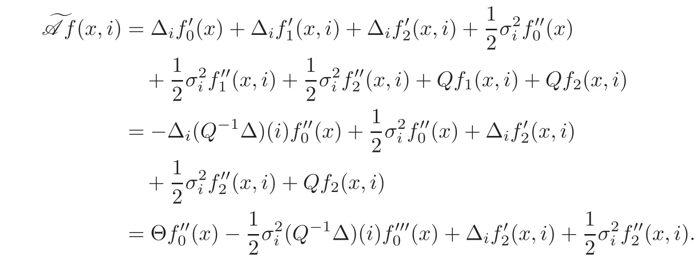
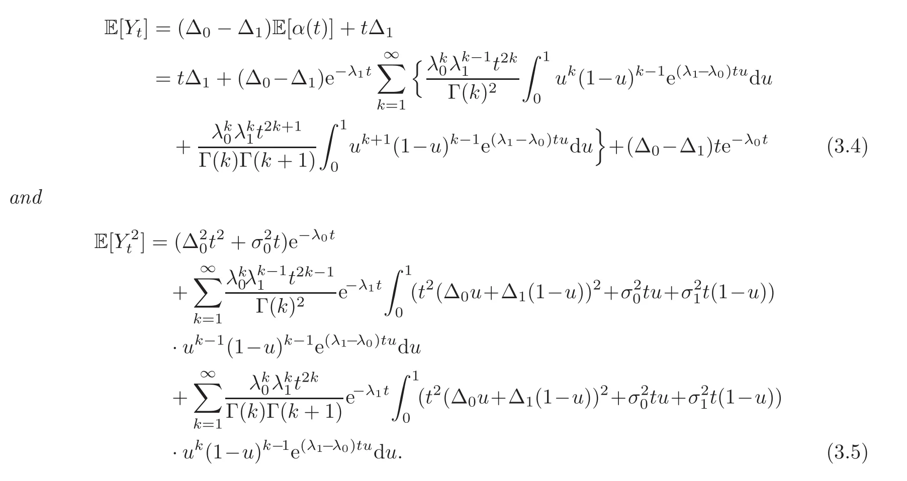
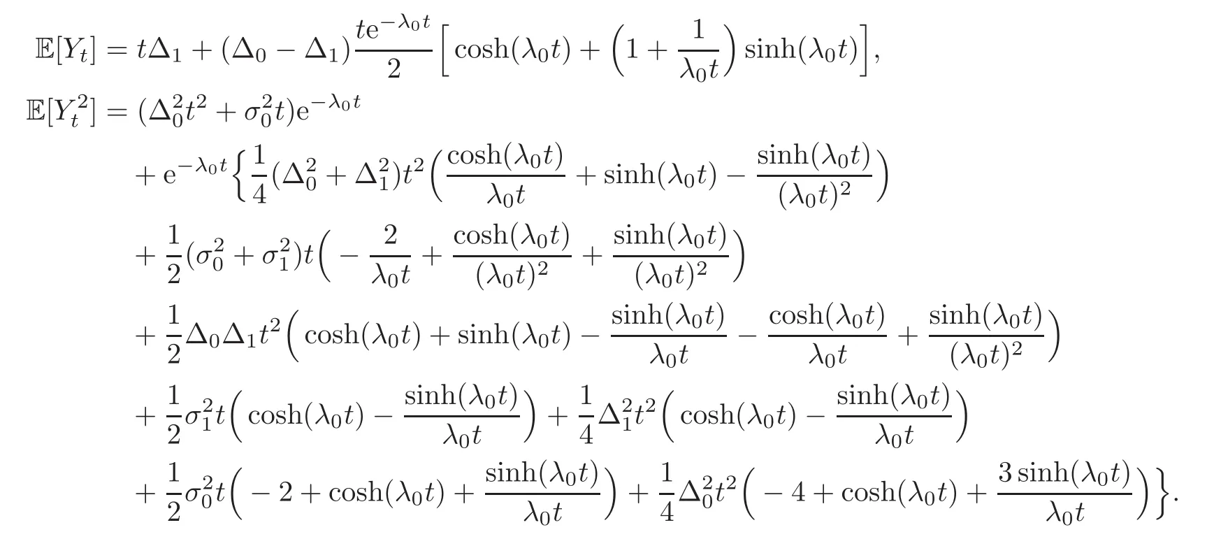
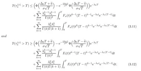
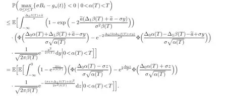
For any 0≤s

Hence

Fix time t>0,and let τ1< τ2< ···,τMbe the jumping time of(Λt)during the period(0,t).Set τM+1=t,τ0=0.Then r 7→pµΛr+12p(p−1)σ2Λris continuous during(τk,τk+1)for k=0,···,M.Hence(2.3)implies that

and further

for k=0,···,M.Due to the continuity of r 7→ EP1Xpr,we obtain that

and hence

According to[1,Proposition 4.1],there exist constants 0

Consequently,

which is the desired conclusion.

Now we proceed to study the recurrent property of(Xt,Λt).Due to(1.3),Yt=lnXtis well-defined for t≥0 a.s.and satisfies the SDE(2.2).It is obvious that the recurrent property of(Xt,Λt)is equivalent to that of(Yt,Λt).We shall use the Lyapunov method to justify the recurrent property of(Yt,Λt).

Proof of Theorem 1.2(i)We shall use the method of[18,Section 3].Set h(x)=|x|−2and g(x)=|x|−3for|x|≥ 1.Define

Then

Let us first consider the casethere exist ε>0,r1>1 such thatand

According to the Fredholm alternative,there exists a constant κ >0 and a vector(ξi)i∈Sso that

Setting f(x,i)=h(x)+ξig(x)for x>0,we derive that

Take Y0=y>r2and Λ0=i0so that f(y,i0)0;Yt=K},K>r2,τ=inf{t>0;Yt=r2}.By Dynkin’s formula,

Letting t→+∞,we get

which yields further that

in the last step of which we have used the decreasing property of the function h(x)+ξming(x)on[r2,+∞).Invoking the fact τK→+∞ as K ↑+∞ a.s.,(2.5)yields that

which implies that(Yt,Λt)is transient.

Analogously,we can prove that(Yt,Λt)is also transient whenby using the same Lyapunov function f(x,i)but studying its behavior on x<0.

(ii)Now we consider the caseWe shall apply the technique used in[14].Setand

Then,Θ >0 due to the Fredholm alternative,and Θfor x0 by direct calculation.Define f1(x,i),f2(x,i)by

which are well-defined due to the factand

Take f(x,i)=f0(x)+f1(x,i)+f2(x,i)for|x|6=0,i∈S.Then

Next,we shall show further that whenor equivalently(Yt,Λt),is null recurrent.To this aim,we take 1

where ξiis determined by Qξ(i)= −∆ifor each i∈ S satisfying further ξi>0,i∈ S.Direct calculation yields that

for x>0,i∈S.As p,q∈(1,2),it is easy to obtain that there exist constants r1,K>0 such that

Let

where C>0 satisfying u(r1,i)=g(r1,i)−C<0 for all i∈S.Set

Since h(m,i)−Rmu(m,i)≥ 0,and h(r1,i)−Rmu(r1,i)≥ 0 for every i∈ S and m large enough,we obtain

Letting m→+∞,(2.6)yields that

Hence,(Yt,Λt)is not positive recurrent.However,we have shown(Yt,Λt)is recurrent.In all,(Yt,Λt)is null recurrent.The proof of Theorem 1.2 is complete.

3 Some Quantitative Properties of SGBM

In this section,we shall exploit the quantitative properties of the process(Xt,Λt).Throughout this section,we only consider the case that(Λt)is a Markov chain on S={0,1}.To emphasize this fact,in this section we denote the Q-matrix of(Λt)by

where λ0,λ1are two positive constants.We calculate the moments of lnXtin Subsection 3.1,and provide the estimate of the first passage probability of(Xt)in Subsection 3.2.

3.1 Moments of lnXt

Let us introduce some notations used in the sequel.Assume that Λ0=i for i=0 or 1.Set

Let τk= ζk− ζk−1for k ≥ 1 with ζ0:=0,then(τk)k≥1are mutually independent random variables,and τ2kand τ2k−1are both exponentially distributed with parameters λ1−iand λi,respectively.Let α(t)and β(t)denote respectively the time spent by the process(Λt)at the states Λ0and 1−Λ0up to the time t.Let N(t)be the total number of transition between state 0 and 1 happened during(0,t).

According to[16],the distribution of the sojourn time α(t)when Λ0=0 is

Now we consider the geometric mean of the process(Xt).Let

Recall that∆0and∆1are defined by(1.5).Due to the independent increasing property of Brownian motion,we can rewrite Ytin the form

where ξ(u)and η(u)(for u>0)are mutually independent normally distributed random variables with mean 0 and variance u,and ξ(u),η(u)are independent of the process(Λt).

Proposition 3.1 Assume Λ0=0.For t>0,it holds

In particular,when λ0= λ1,

ProofBy the distribution of α(t),ξ(u),η(u),we get(3.4)by direct calculation.By the formula(3.3),due to the independence of ξ(u)and η(u),we get

Then we obtain(3.5)according to the distribution of α(t).Using the Taylor expansion of functions cosh(x)and sinh(x)the formulas of E[Yt]and E[Y2t]in the case λ0= λ1can be obtained.

Using the same method,every n-th order moments of Ytcan be calculated.

Proposition 3.2 Assume Λ0=0.Then

Proof According to the results[25,Theorems 6–7],it holds that

Hence we have

Then by the formula(3.3),we can get the desired results by direct calculation.

3.2 First passage probability of(Xt)

For fixed x>a>0,let

What we are interested in is the probability

Although the first passage probability is very useful,the calculating of it is very difficult.Only for several simple cases,explicit formulas exist.For example,explicit formula exists for one-dimensional Brownian motion and piecewise monotone functionals of Brownian motion(see[26]).To deal with general diffusion processes,one has to rely on some numerical approximation schemes.The regime-switching geometric Brownian motion provides us a simple example to see the difference between the study of first passage probability for diffusion processes and the study of the first passage probability for regime-switching diffusion processes.Below,one can easily find that the switching of(Λt)causes new difficulty in calculating the first passage probability.

In this subsection,we consider first the case σ0= σ1= σ >0,then the case σ06.When σ0= σ1= σ,one gets by(1.4)that

For fixed T>0,let

Then

Indeed,by(3.9),we get,when t≤ β(T),

and when β(T)

Similarly,we can prove the first inequality of(3.10).

and

Theorem 3.1 Assume σ0= σ1= σ >0,∆1≥ ∆0.Suppose that the process(Λt)starts from 0,i.e.,Λ0=0 a.s.For every T>0,it holds

Proof By(3.8)and(3.10),we get

Due to the independence of(Λt)and(Bt),

where FΛ=σ(Λt;t≤T).According to the well-known results on the first passage probability of Brownian motion(see for example,[23,p.375]),

Consequently,if α(T)=T,then

If 0<α(T)

Under the assumption Λ0=0,one has P(α(T)>0)=1.Then,invoking the distribution of α(T)and the definition of Fu(t),we can get(3.11).By a similar argument,we can get(3.12),and the proof is completed.

Now we consider the first passage probability of(Xt)when σ06= σ1.Note that σ0,σ1stand for the volatility,so it is not restrictable to assume that σ0,σ1>0.

Proposition 3.3 Assume that σ0> σ1>0.For each 00,it holds

where η0is a standard normally distributed random variable,and is independent of(Bt,Λt).

Proof For clarity of the idea,let us introduce a probability space(Ω,P).Let Ω = Ω1×Ω2=C([0,∞);R × S).Then there exists a probability measure P=P1× P2on Ω such that ω =(ω1(·),ω2(·))satisfying thatis a Brownian motion under P1on Ω1and(ω2(t))is a Q-process with Q-matrixnder P2on Ω2.Set Bt(ω)= ω1(t)and Λt(ω)= ω2(t).Then under P,(Bt)and(Λt)satisfy the condition used in the definition of the process(Xt,Λt).Moreover,

Recall the definition of ζkin the beginning of Subsection 3.1.For t∈ (ζ2k,ζ2k+1],we have

where B(1)(t)and B(2)(t)are independent normally distributed random variables for each t>0,which satisfies

For N∈N and k∈N such thatkN≤T,set

Then(Yk)kare Gaussian random variables satisfying

Moreover,for every k

Hence

Then(Zk)kare Gaussian random variables with

Therefore,according to Slepian’s lemma(see[12,p.74]),we have

Then applying the symmetry of the Brownian motion,we get the desired conclusion.

Remark 3.1 According to this proposition,we can transform the situation σ06= σ1to the situation σ0= σ1via Slepian’s lemma.Combining with Theorem 3.1,we can obtain an upper bound of P(τ(x)a>T)when σ06= σ1.

AcknowledgementThe author is grateful to Professors Mu-Fa Chen and Yong-Hua Mao for their valuable discussion.