Error Analysis on Hérmite Learning with Gradient Data∗

Baohuai SHENGJianli WANGDaohong XIANG

Abstract This paper deals with Hérmite learning which aims at obtaining the target function from the samples of function values and the gradient values.Error analysis is conducted for these algorithms by means of approaches from convex analysis in the framework of multi-task vector learning and the improved learning rates are derived.

Keywords Hérmite learning,Gradient learning,Learning rate,Convex analysis,Multitask learning,Differentiable reproducing kernel Hilbert space

1 Introduction

We considered Hérmite learning with gradient vectors(see[1–4])in this paper.It can produce a smoothness function when the function value samples and gradient data is provided.

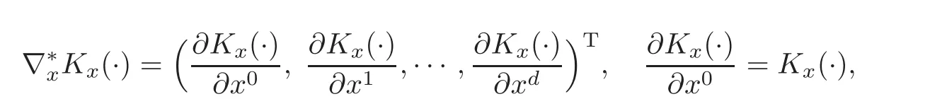
Let X be a compact subset of the Euclidean space Rdon which the learning or function approximation is considered.For each x=(x1,x2,···,xd)T∈ X,the gradient of function f:X→R at x is denoted by the vector

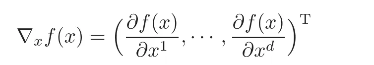
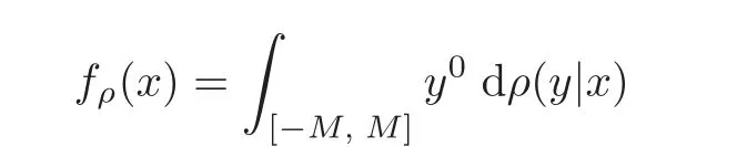
if the partial derivative for each variable exists.It is known(see[2])that the essence of Hérmite learning is to obtain the regression function fρ(x)=RRydρ(y|x)from samples z=whereare drawn independently according to ρ(x,y)= ρ(y|x)ρX(x)and eyi≈ ∇f(xi).

Let K:X×X→R be a Mercer kernel which is continuous,symmetric and positive semidefinite,which means that the matrixis positive semi-definite for any finite set of points{x1,···,xl} ⊂ X.The associated reproducing kernel Hilbert space(RKHS)HKis defined(see[5–7])as the completion of the linear span of the set of the function{Kx=K(x,·):x∈X}with the inner product given by

Let L2(µ)be the class of all square integrable functions with respect to the mesure µ with the norm

Define the integral operator LKas

Since K is a positive semi-definite,LKis a compact positive operator.Let λkbe the k-th positive eigenvalue of LK(f)and φk(x)be the corresponding continuous orthonormal eigenfunction.Then,by Mercer’s theorem,for all x,y ∈ X,there holds

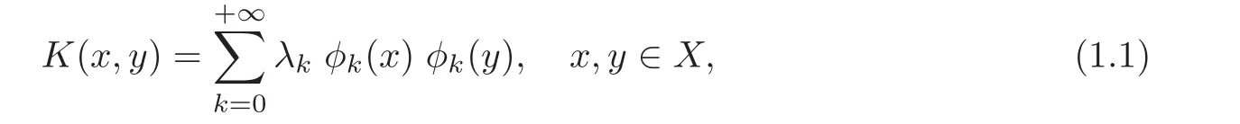
where the convergence is absolute(for each x,y∈X)and uniform on X×X.Then we know(see[8–9])

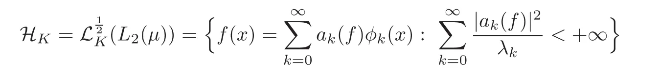
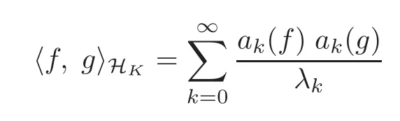
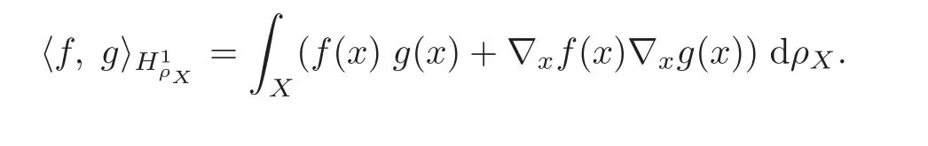
with inner product

When X is a compact set,there is a constant k>0 such that

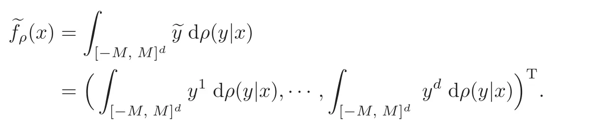
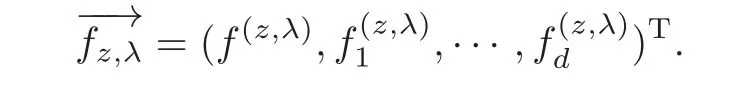
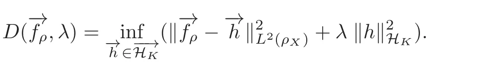
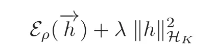
Let M>0 be a given positive real number and Y=[−M,M]d+1.We denote by y ∈ Y as y=(y0, ey)with ey=(y1,y2,···,yd)Tand

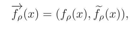
where

and

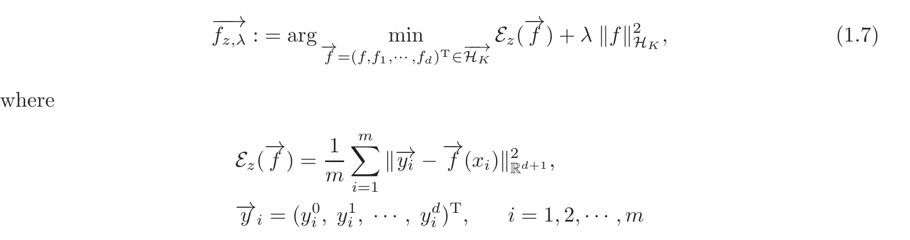
where λ >0 is the regularization parameter,k ·kRdis the usual norm of the Euclidean space

The representer theorem for scheme(1.3)was provided in[1],which showed that the minimization over the possibly infinite dimensional space HKcan be achieved in a finite dimensional subspace generated by{Kxi(·)}and their partial derivatives.The explicit solution to(1.3)and an upper bound for the learning rate with the integral operator approach were given in[2].

We notice that the problem of learning multiple tasks with kernel methods has been a developing topic(see[10–14]).The representer theorem for these frameworks have been given,but the results of convergence quantitative analysis are relatively few,and very effective methods for bounding the convergence rates does not appear.An aim of the present paper is to show that model(1.3)is among the group of the multiple tasks.For this purpose,we rewrite model(1.3)from the view of vector valued functions.

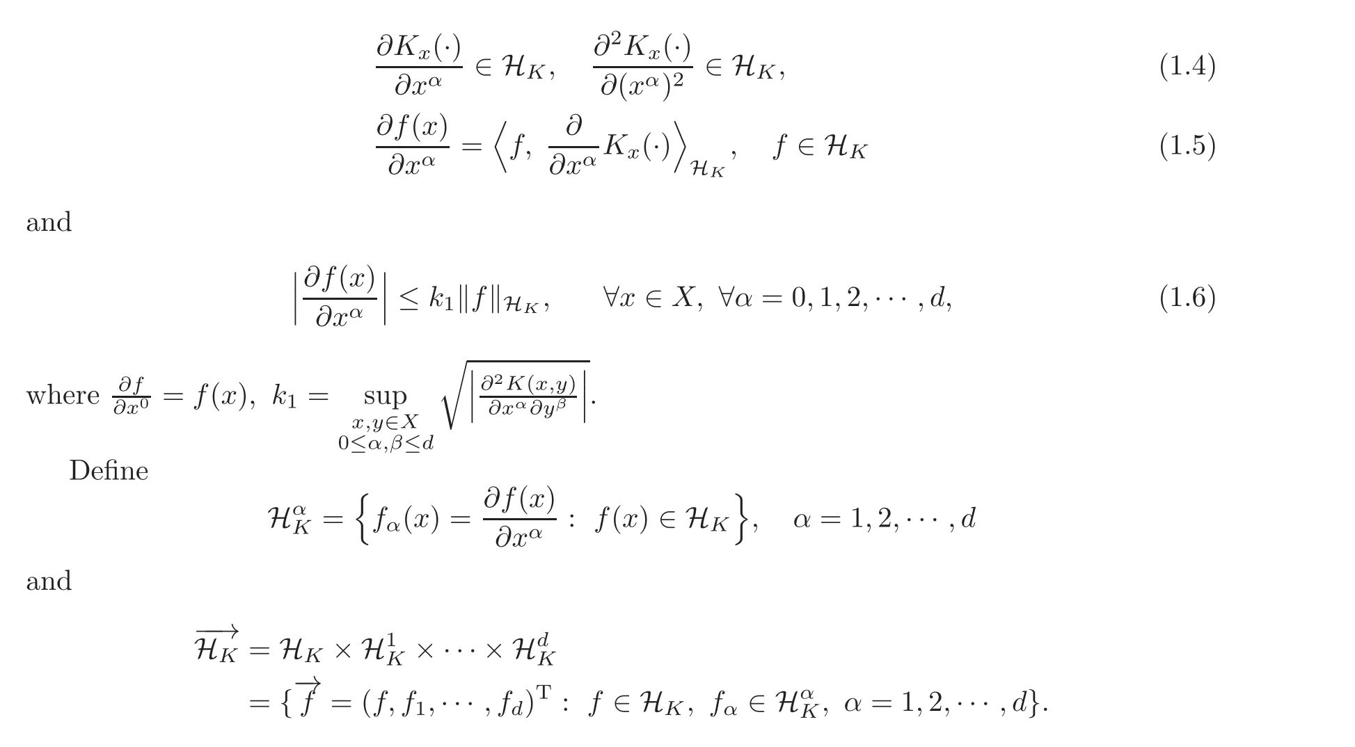
Let C(1)be the class of all the real functions f(x)defined on X with continuous partial derivatives and C(2)(X)denote the class of all the real functions f(x)defined on X with continuous partial derivativesfor α =1,2,···,d.By K ∈ C(2)(X × X),we mean all the partial derivativesthat are continuous on X × X.By[15–17]we know that if the kernels K(x,y)have the form of(1.1)and K(x,y)∈C(2)(X×X),then,HKcan be embedded into both C(1)(X)and C(2)(X),and for any given x ∈ X and all α =1,2,···,d,the following relations hold:

Then,(1.3)can be rewritten as

and

Algorithm(1.7)is neither the same as the usual least square regression(see[18–21]),nor the current multitask learning model since it uses the penaltyHowever,it is really a concrete example of multitask learning models,the study method of its performance can provide useful reference for the research of other multitask models.This is the first motivation for writing this paper.On the other hand,such approaches may provide a way of thinking for dealing with other gradient learning models.The structure of model(1.7)is close to the usual least square learning models,this fact creates an opportunity of studying the gradient learning with existing methods,e.g.,the convex analysis method(see[20–24]).This is the second motivation for writing this paper.

We form an improved convex method with the help of Gâteaux derivative and the optimality conditions of convex functions and use it to bound the convergence rates of model(1.7).To show the main results of the present paper,we restate the notion of covering number.

For a distance space S and a real number η >0.The covering number N(S,η)is defined to be the minimal positive integer number l such that there exists l disks in S with radius η covering S.

We call a compact subset E of a distance space(B,k·kB)logarithmic complexity exponent s≥0 if there is a constant cs>0 such that the closed ball of radius R centered at origin,i.e.,

satisfies

We now give the following Theorem 1.1.

Theorem 1.1 Let K(x,y)be a Mercer-like kernel satisfying Kbe the solution of(1.7)and C=512(d+1)3M.If Hkhas logarithmic complexity exponent s ≥ 0 in the uniform continuity norm and 0<δwith confidence 1−δ,we havethen,for any 0< δ<1

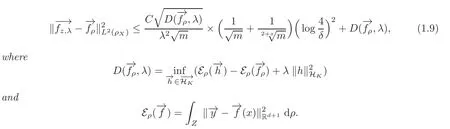
We now give some comments on(1.9).

If ρ is perfect(see[2]),i.e.,

(2)By Lemma 2.2 afterward we have

As usual,we assume that there are given constants c>0 and 0< β <4 such thatcλβifis density in L2(ρX).In this case,if s=0,then we have by(1.9)that

Further,if λ=m−θand 0<θ<,then,we have by(1.10)the following estimate

(3)Define a new integral operator

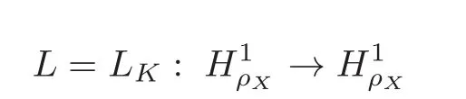
associated with K and ρXby

Let LrKbe defined as

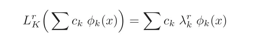
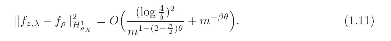
for r>0.Then,by taking λ =8(d+1)k2log()m−β,with confidence 1−δ,we have(see[2])

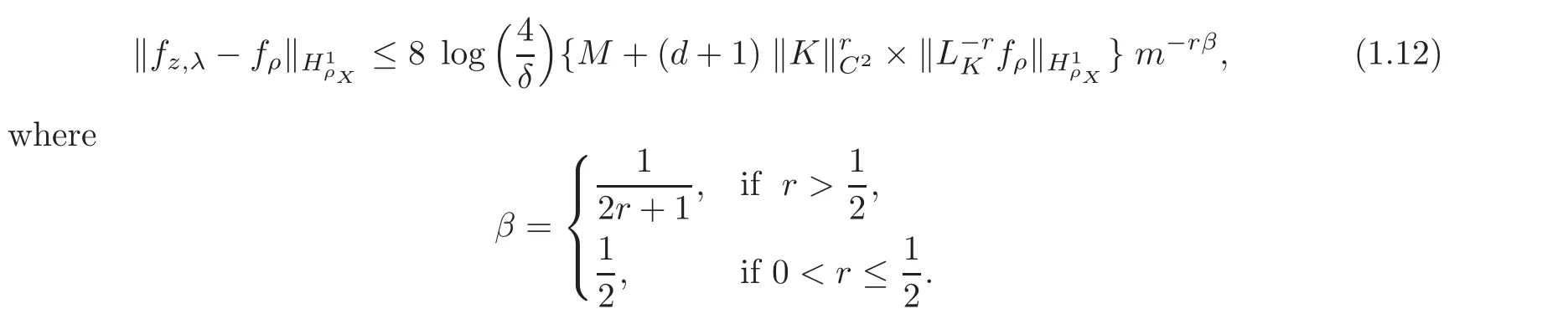
It is easy to see that(1.11)sharps(1.12).

2 Proofs

To show Theorem 1.1,we need the notation of the Gâteaux derivative and some related lemmas.

Let(H,k·kH)be a Hilbert space,F(f):H → R∪{∓∞}be a real function.We say F is Gâteaux differentiable at f ∈ H,if there is a ξ∈ H such that for any g ∈ H,there holds

and write ∇fF(f)= ξ as the Gâteaux derivative of F(f)at f.

Lemma 2.1 Let F(f):H→R∪{∓∞}be a function defined on Hilbert space H.Then,we have following results:

(i)If F(f)is a convex function,then,F(f)attains minimal value at f0if and only if∇fF(f0)=0.

(ii)If F(f):H → R∪{∓∞}is a Gâteaux differentiable function,then,F(f)is a convex on H if and only if for any f,g∈H we have

Proof We have(i)from Proposition 17.4 of[25]and we have(ii)from Proposition 17.10 and Proposition 17.12 of[25].

and the equation

Proof Since equality

holds for any a,b∈Rd+1,we have

Then,we have the following Lemma 2.3.

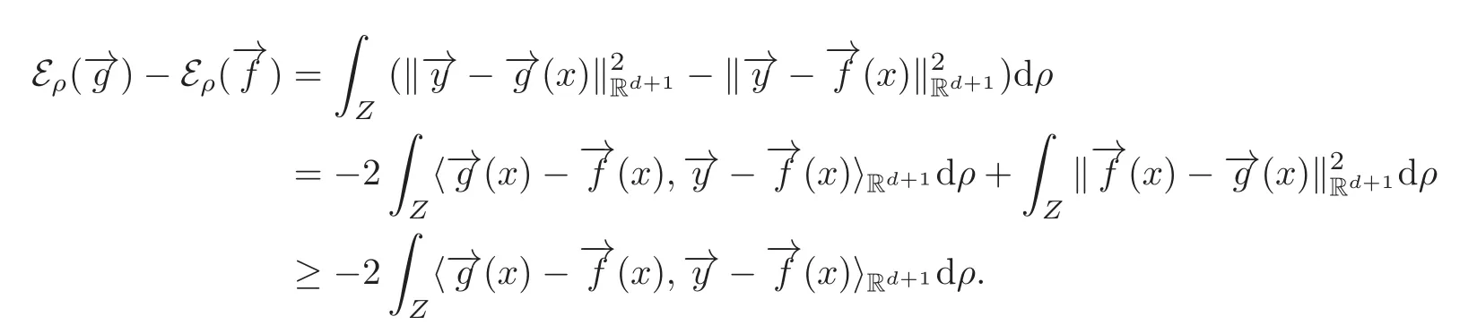
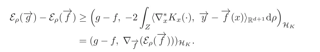
Proof By the equality

we have

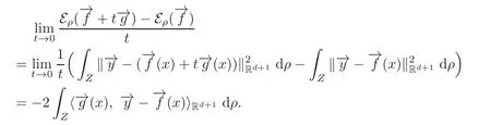
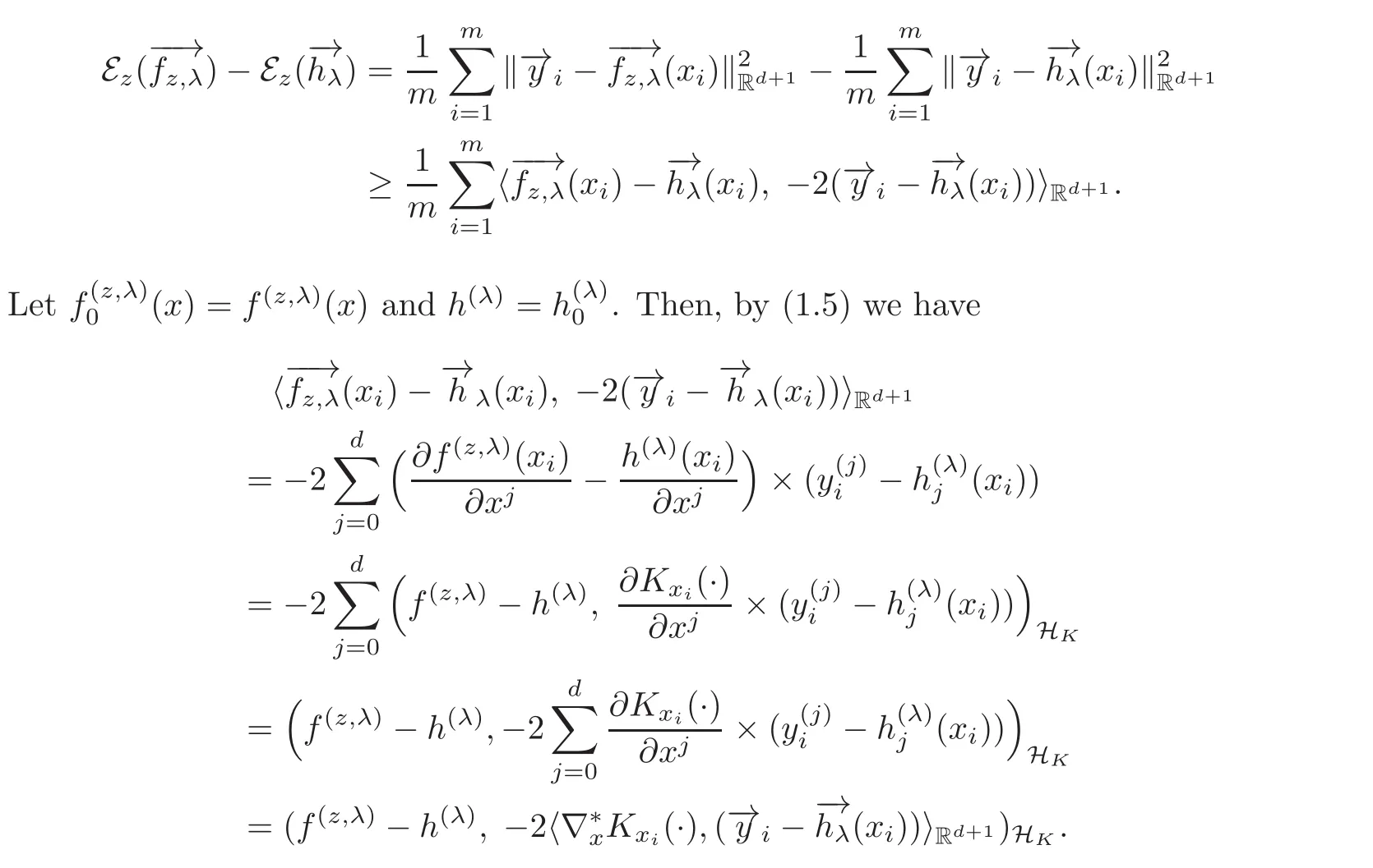
Take g0(x)=g(x),f0(x)=f(x).Then,by(1.5)we have

It follows

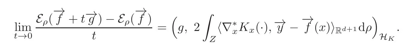
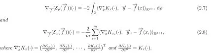
(2.7)thus holds.(2.8)can be proved in the same way.

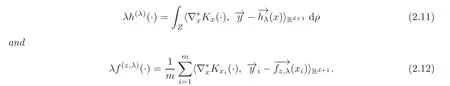
where we have used the fact that

(2.11)thus holds.(2.12)can be proved in the same way.

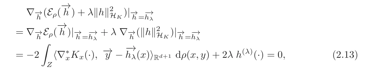
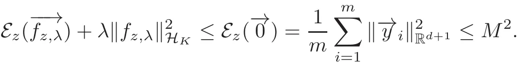
Lemma 2.5(2.6)has a unique solutionand(1.7)has a unique solutionThey satisfy the following inequalities:

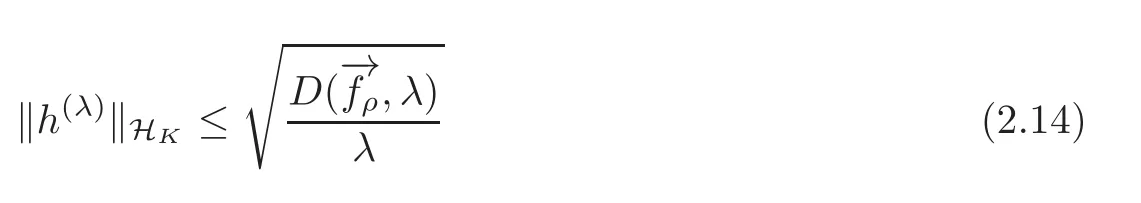
and

Since(2.10),we have

Therefore,by(2.7)we have

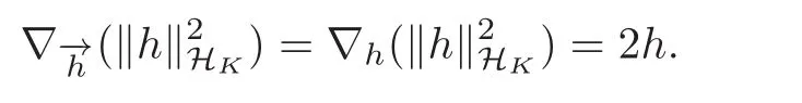
By the definition ofwe have

(2.14)then holds.By the definition ofwe have

(2.15)thus holds.

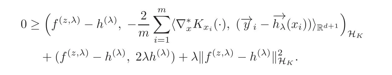
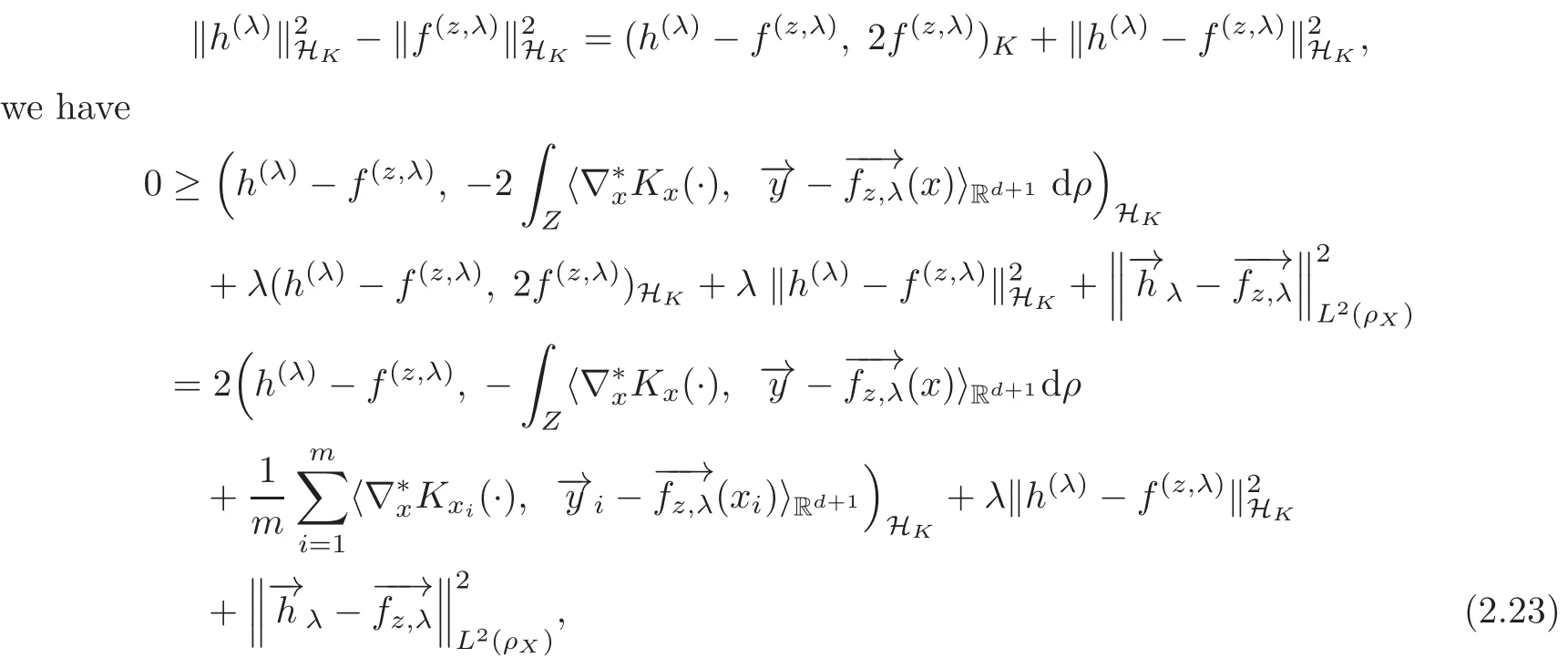
Proof By(2.9),we have

Therefore,

Since HKis a Hilbert space,the parallelogram law shows

It follows by(2.17)–(2.18)that

By(2.11)we have

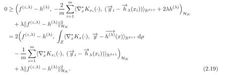
(2.19)gives(2.16).

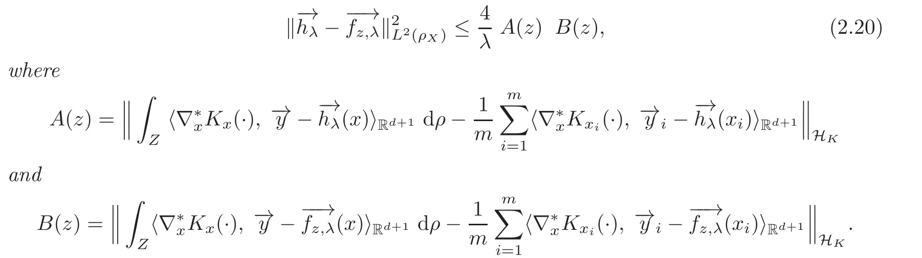
Proof By(2.9)we have

Further,by(2.21)and the equality

where we have used(2.12).By Cauchy’s inequality we have

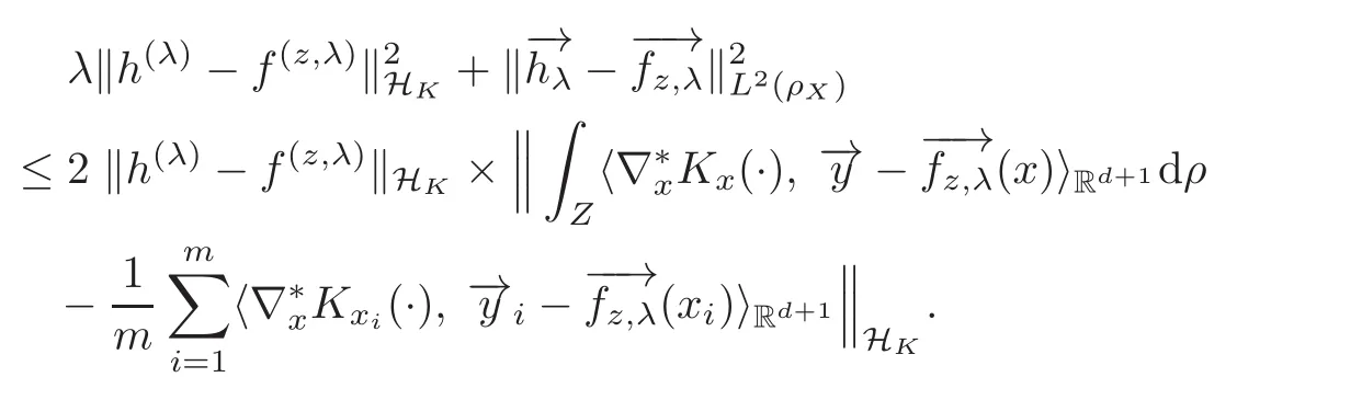
Above inequality leads to

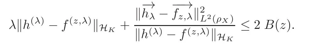
It follows that

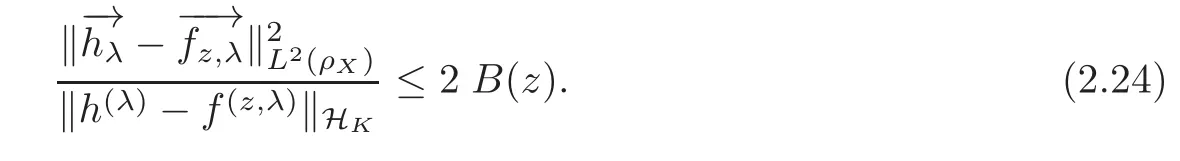
By(2.16)and(2.24)we have(2.20).

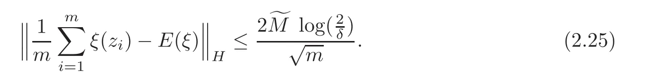
Lemma 2.8 (see[19])Let(H,k·k)be a Hilbert space and ξ be a random variable on(Z,ρ)with values in H.Assume thatlmost surely.be independent samples drawers of ρ.For any 0< δ<1,with confidence 1 − δ,

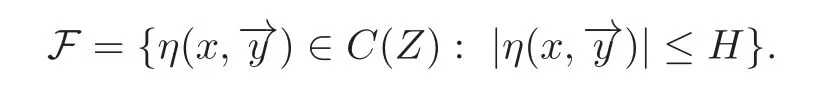
Lemma 2.9 (see[6])Let F be a family of functions from a probability space Z to ℜ and d(·,·)be a distance on F.Let U ⊂ Z be of full measure and constants H,p>0 such that

(i)|ξ(z)|≤ H for all ξ∈ F and all z ∈ U,and

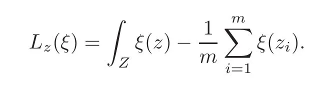
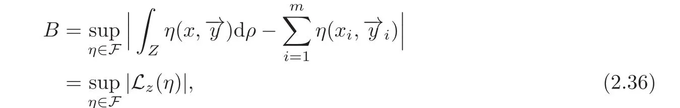
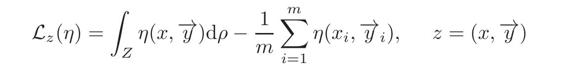
(ii)|Lz(ξ1)− Lz(ξ2)|≤ p d(ξ1, ξ2)for all ξ1,ξ2∈ F and all z ∈ Um,where

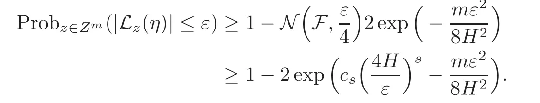
Then,for all ǫ>0,

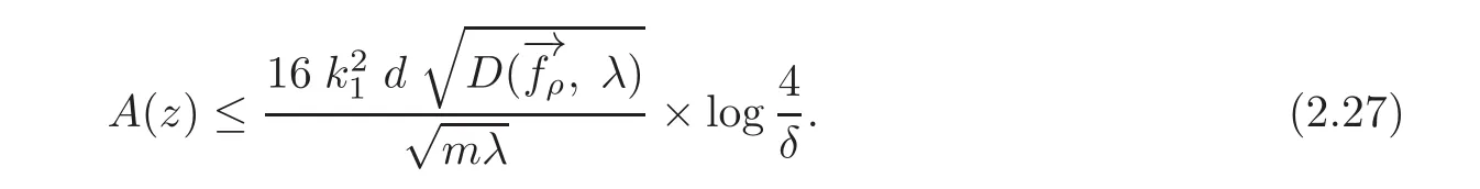
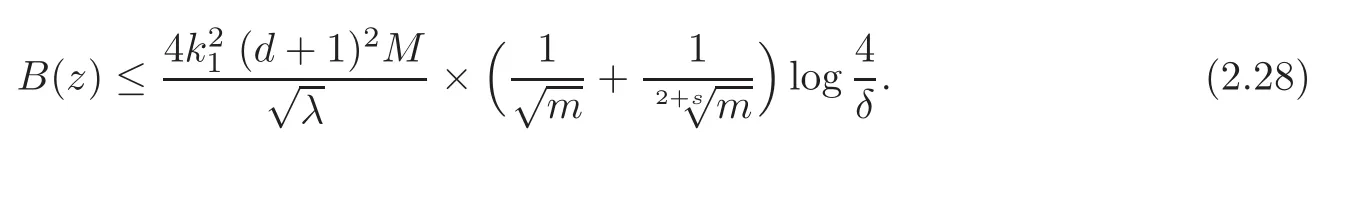
Lemma 2.10 Under the conditions of Theorem 1.1,we have the following two estimates:

(1)For any δ∈(0,1),with confidence 1−we have

(2)For any δ∈ (0,1)and 0< δ,with confidence 1−,we have

Proof of(2.27)Take

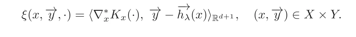
Since

we have

By(1.5),we have

Furthermore,by(2.14)we have

By(2.32)and(2.25),we have(2.27).

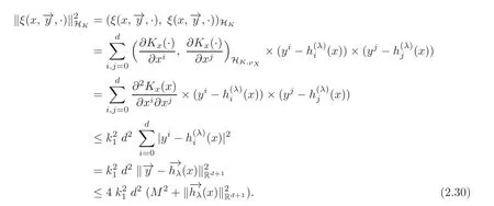
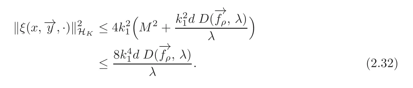
Proof of(2.28)By the definition of k·kHK,we have

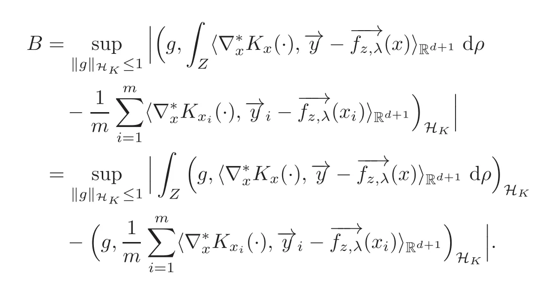
By(2.10),we have

and by(2.15),we have

Therefore,

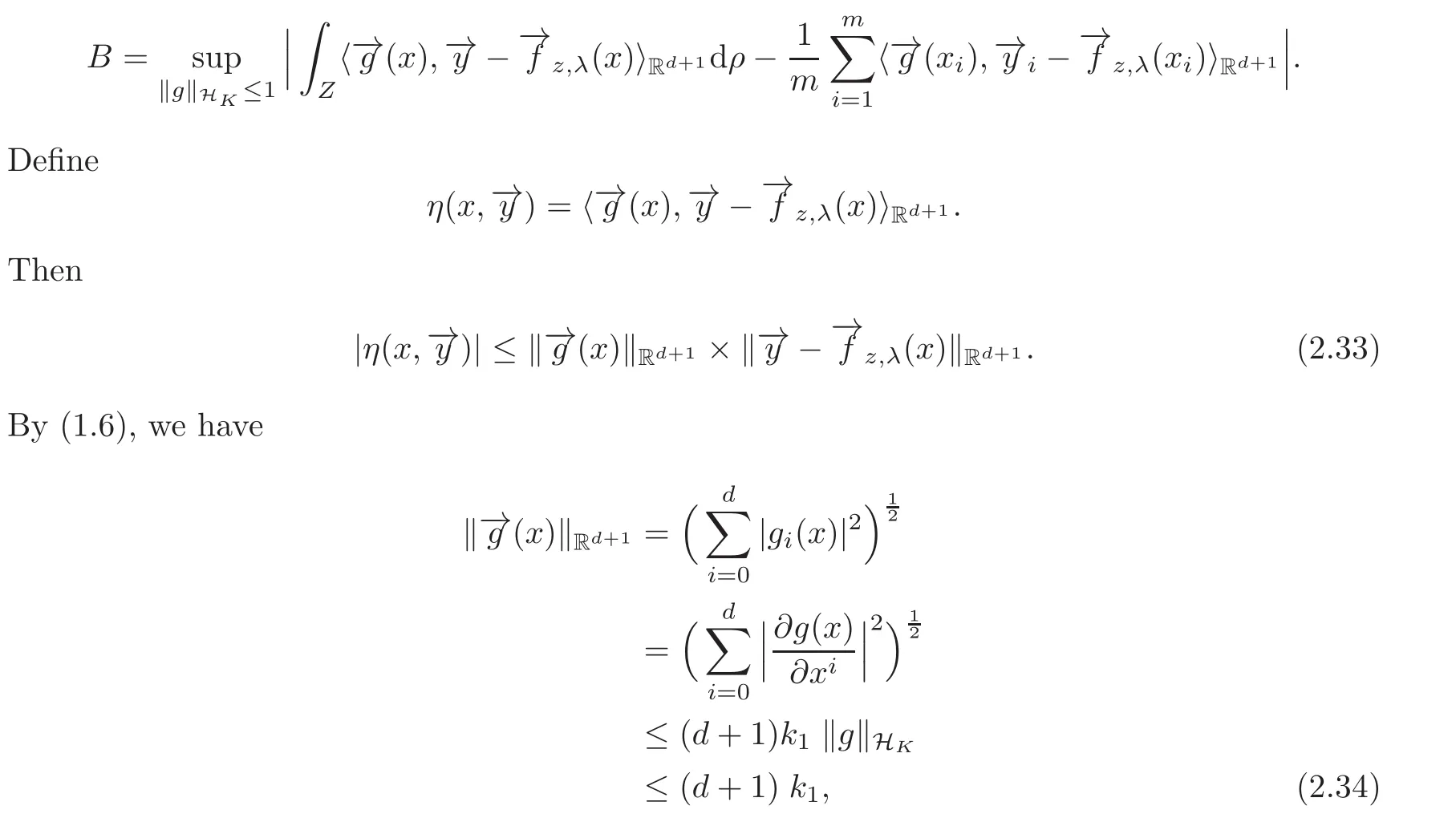
Take

Then,

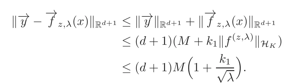
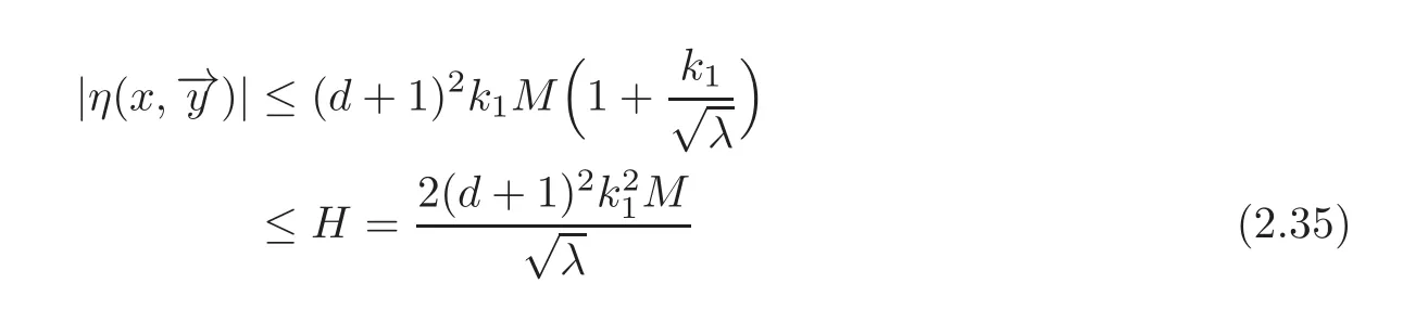
where

satisfies the inequality

By Lemma 2.9,we have for any ε>0

Take

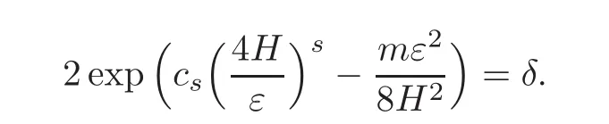
Then,we have

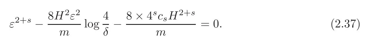
Notice that there is the famous lemma(see[26]).

Let c1>0,c2>0 and u>t>0.Then the equation

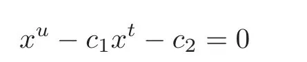
has a unique positive zero x∗.In addition,

By(2.37)–(2.38),we have

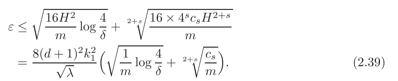
By(2.36)and(2.39),we have(2.28).

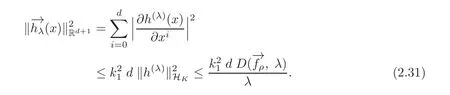
Lemma 2.11 For any δ∈ (0,1),with confidence 1 − δ,we have

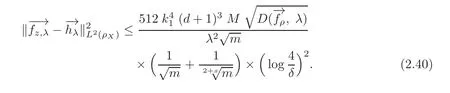
Proof By(2.20),we have

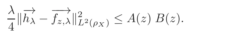
Then,

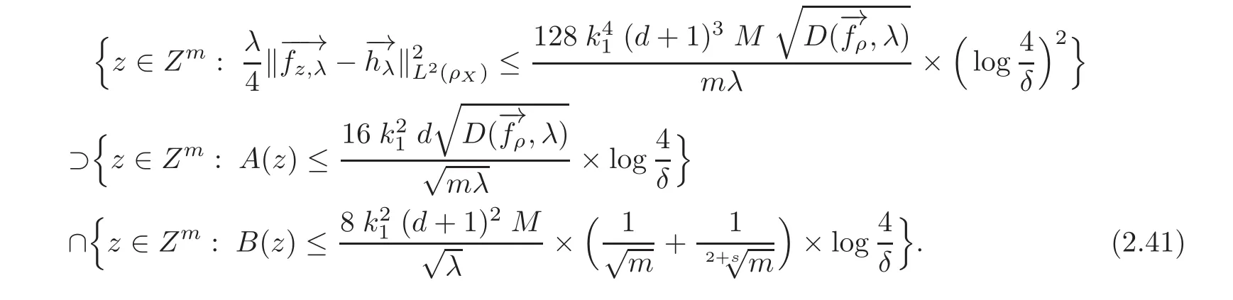
By(2.27)–(2.28)and(2.41),we have(2.40).

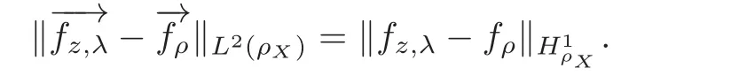
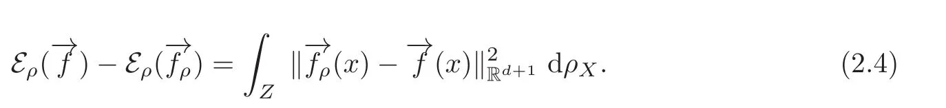
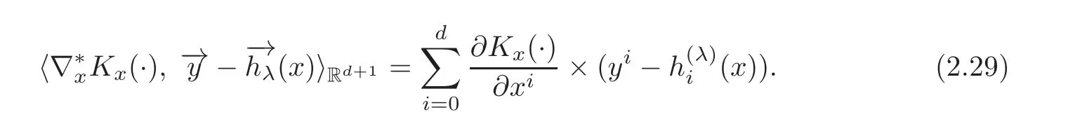
Proof of(1.9)By the definition of−→

hλ,(2.3)–(2.4)we have

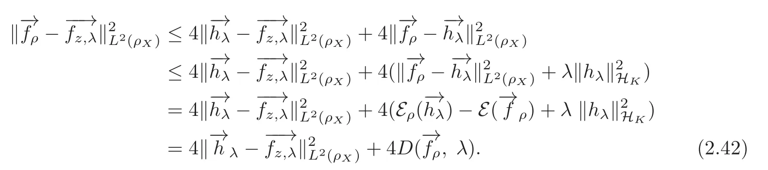
(2.40)and(2.42)give(1.9).