
Model Selection Consistency of Lasso for Empirical Data∗
2018-10-18 02:54:16YuehanYANGHuYANG
Yuehan YANG Hu YANG
Abstract Large-scale empirical data,the sample size and the dimension are high,often exhibit various characteristics.For example,the noise term follows unknown distributions or the model is very sparse that the number of critical variables is fixed while dimensionality grows with n.The authors consider the model selection problem of lasso for this kind of data.The authors investigate both theoretical guarantees and simulations,and show that the lasso is robust for various kinds of data.
Keywords Lasso,Model selection,Empirical data
1 Introduction
Tibshirani[14]proposed the lasso(least absolute shrinkage and selection operator)method for simultaneous model selection and estimation of the regression parameters.It is very popular for high-dimensional estimation due to its statistical accuracy for prediction and model selection coupled with its computational feasibility.On the other hand,under some sufficient condition the lasso solution is unique,and the number of non-zero elements of lasso solution is always smaller than n(see[15–16]).In recent years,this kind of data has become more and more common in most fields.Similar properties can also be seen in other penalized least squares since they have a similar framework of solution.
Consider the problem of model selection in the sparse linear regression model

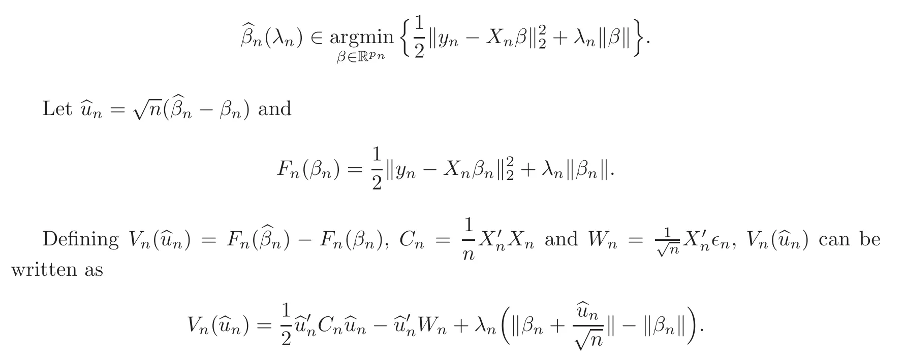
where the detail setting of the data can be found in the next section.Then the lasso estimator is defined as
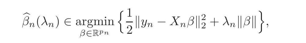
where λnis the tuning parameter which controls the amount of regularization.Set≡ {j ∈{1,2,···,pn}:bβj,n6=0}to select predictors by lasso estimatorConsequently,andboth depend on λn,and the model selection criteria results in the correct recovery of the set Sn≡ {j ∈ {1,2,···,pn}:βj,n6=0}:

On the model selection front of the lasso estimator,Zhao and Yu[22]established the irrepresentable condition on the generating covariance matrices for the lasso’s model selection consistency.This condition was also discovered in[11,20,23].Using the language of[22],irrepresentable condition is defined as|C21sign(β(1))|6 1 − η,where sign(·)maps positive entry to 1,negative entry to−1 and zero to zero.The definitions of C21and C11can be seen in Section 2.When signs of the true coefficients are unknown,they need l1norms of the regression coefficients to be smaller than 1.Beyond lasso,regularization methods also have been widely used for high-dimensional model selection,e.g.,[2,4,7–8,10,12,17–19,21,24–25].There has been a considerable amount of recent work dedicated to the lasso problem and regularization methods problem.
Yet,the study of model selection problem for empirical data is still needed.Stock data for instance,the Gaussian assumption of the noise term is always unsatisfied for these data.And the critical variables are extremely few contrast to the collected dimensionality.In this paper,we consider this kind of data:The sample size and the dimension are high,but the information of critical variable data is missing(the signs of the true βnand the distribution of the noise terms are unknown)and the model is extremely sparse that the number of nonzero parameter is fixed.This kind of data is common in the empirical analysis hence we called it empirical data.
We consider the model selection consistency of lasso and investigate regular conditions to fit this data setting.Under conditions,the probability for lasso to select the true model is covered by the probability of

where Wn=and Gnis a function of λn,n,q.Above inequality is simple and also easy to calculate its probability.Based on the train of thought of the proof,we analyze the model selection consistency of lasso under easier conditions than the irrepresentable condition for empirical data.In the simulation part,we discuss the effectiveness of lasso.Four samples are given,in which the irrepresentable condition fails for all the settings,but lasso still can select variables correctly in two of them when our conditions hold.
We discuss the different assumptions of noise terms ǫi,nfor model selection consistency.Gaussian errors or the subgaussian errors1e.g.P(|ǫi,n|>t)6 Ce−ct2, ∀t>0.would be standard,but possess a strong tail.One basic assumption in this paper is that,errors are assumed to be identically and independently distributed with zero mean and finite variance.
The rest of the paper is organized as follows.In Section 2,we investigate the data setting,notations,and conditions.We introduce a lower bound to cover the case in which the lasso chooses wrong models when suitable conditions hold.Then,to demonstrate the advantages of this bound,we show the different settings and different assumptions of noise terms in Section 3.We show that the lasso has model selection consistency for empirical data with mild conditions.Section 4 presents the results of the simulation studies.Finally,in Section 5,we present the proof of the main theorem.
2 Data Setting,Notations and Conditions
Consider the problem of model selection for specific data
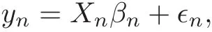
where ǫn=(ǫ1,n,ǫ2,n,···,ǫn,n)′is a vector of i.i.d.random variables with mean 0 and variance σ2,Xnis an n×pndesign matrix of predictor variables,βn∈ Rpnis a vector of true regression coefficients and is commonly imposed to be sparse with only a small proportion of nonzeros.Without loss of generality,write βn=(β1,n,···,βq,n,βq+1,n,···,βp,n)′where βj,n6=0 for j=1,···,q and βj,n=0 for j=q+1,···,pn.Then write=(β1,n,···,βq,n)′and=(βq+1,n,···,βp,n),that is,only the first q entries are nonvanishing.Besides,for any vector α =(α1,···,αm)′,we denote
For deriving the theoretical results,we write Xn(1)and Xn(2)as the first q and the last pn−q columns of Xn,respectively.LetPartition Cnas
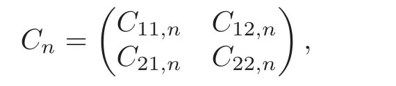
where C11,nis q×q matrix and assumed to be invertible.Set Wn=.Similarly,andindicate the first q and the last pn− q elements of Wn.Suppose that Λmin(C11,n)>0 denotes the smallest eigenvalue of C11,nand consider that q does not grow with n.We introduce the following conditions:
(C1)For j=q+1,···,pn,let ejbe the unit vector in the direction of j-th coordinate.There exists a positive constant 0<η<1 such that

(C2)There exists δ∈ (0,1),such that for all n> δ−1and x ∈ Rq,y ∈ Rpn−q,
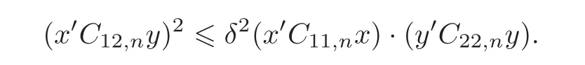
(C1)and(C2)play a central role in our theoretical analysis.Both conditions are easy to satisfy.(C1)for instance,it requires an upper bound on l2-norm,which is much weaker than requires the upper bound on l1-norm,i.e.,irrepresentable condition and variants of this condition[6,9,11,22,25].Another advantage of(C1)is that we do not need the signs of the true coefficients.(C2)requires that the multiple correlations between relevant variables and the irrelevant variables is strictly less than one.It is weaker than assuming orthogonality of the two sets of variables.This condition also has regular appeared many times in the literature,for example,[13].
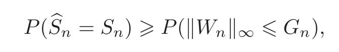
Then we have the following theorem,which describes the relationship between the probability of lasso choosing the true model and the probability of{kWnk∞6 Gn}.Videlicet,it is a lower bound on the probability of lasso picking the true model.
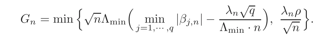
Theorem 2.1 Assume that(C1)–(C2)hold andSet ρ ∈ (0,1).We have
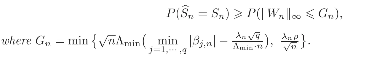
Remark 2.1 Theorem 2.1 is a key technical tool in the theoretical results.It puts a lower bound on the probability of lasso selecting the true model,and this bound is intuitive to calculate.Besides that,considering about Gn,it is easy to find out that there exists a lower bound of non-zero coefficientsThis bound can be controlled by the regularization parameter λn.It is also a regular assumption in the literature that the non-zero coefficients cannot be too small.
Remark 2.2 According to the proof of Theorem 2.1,we can find that it is also directly to obtain the sign consistency of the lasso(see the latter part of the proof).Besides,Theorem 2.1 can be applied in a wide range of dimensional setting.We will discuss the behavior of the lasso on model selection consistency under different settings in the next section.
3 Model Selection Consistency
Now we consider the decay rate of the probability of{kWnk∞>Gn}.Different dimensions and different assumptions of noise terms are discussed in this section.
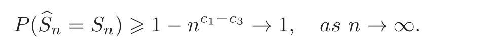
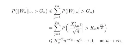
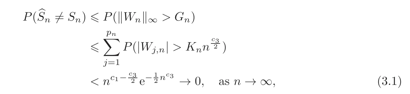
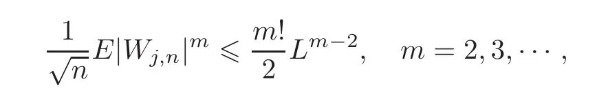
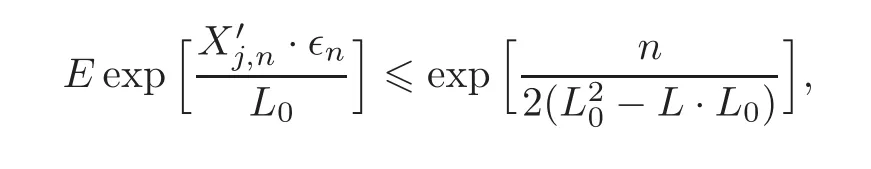
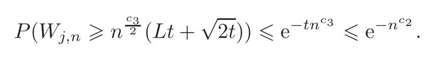
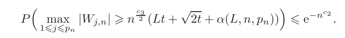
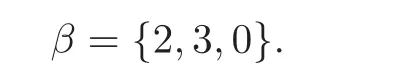
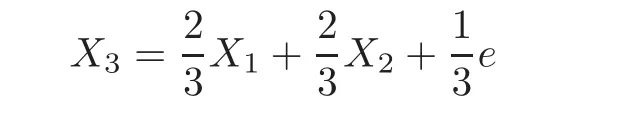
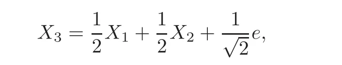
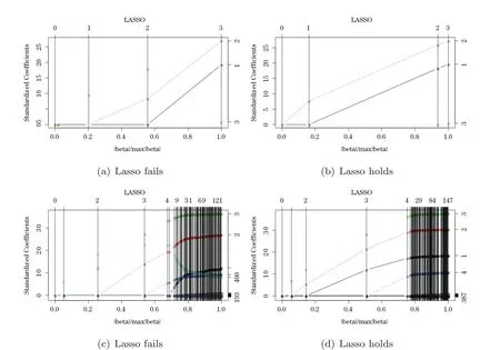
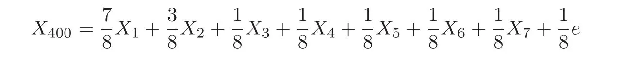
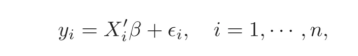
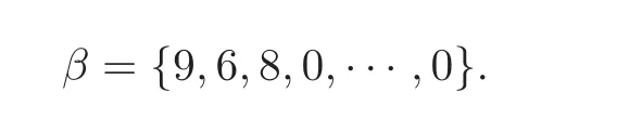
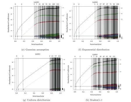
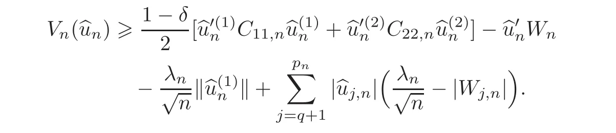
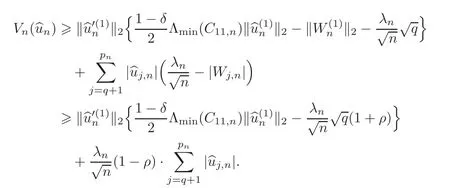
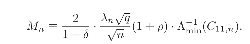
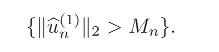
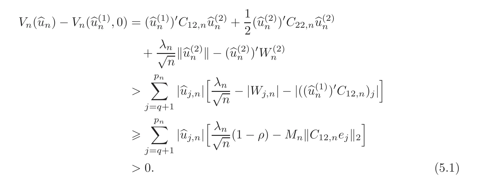
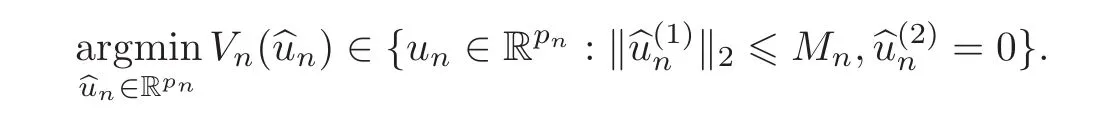
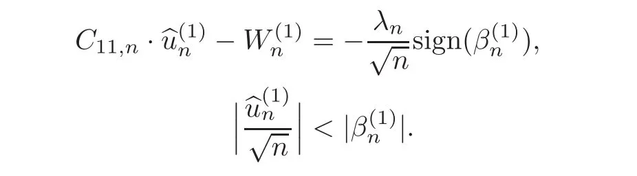
First,we consider general dimensional setting,i.e.,pn=O(nc1)where 0 Before discussing the detail rate of the probability of lower bound,we give the following regular condition: It is a typical assumption in sparse linear regression literature.It can be achieved by normalizing the covariates(see[9,22]). In this part,we consider the general dimensional setting where pnis allowed to grow with n and show the model selection consistency of lasso as follows. Theorem 3.1 Assume that ǫiare i.i.d random variables with mean 0 and variance σ2.Suppose that(C1)–(C3)hold.For pn=O(nc1)where 0 Proof Following the result in Theorem 2.1,we have where Applying the setting of Theorem 3.1,hence for n→∞, Then there exists a positive constant Knthat If(C3)holds,by Markov’s inequality,we easily get The proof is completed. The proof of Theorem 3.1 states that in this setting,lasso is robust and selects the true model with regular restrains.Similarly,if we consider the classical setting where p,q and β are fixed when n→∞,then we have the following result. Corollary 3.1 For fixed p,q and β,under regularity assumptions(C1)–(C3),assume that ǫiare i.i.d random variables with mean 0 and variance σ2.If λnsatisfies that→ ∞ andwhen n→∞,then Similar with the argument of Theorem 3.1,Corollary 3.1 can be proved directly by Markov’s inequality,hence the proof is omitted here. Besides,if we assume that the noise term follows the Gaussian assumption,under the same setting of Theorem 3.1,then we have where the last inequality holds because of the Gaussian distribution’s tail probability bound:P(|ǫi|>t)<∀t>0.It can be relaxed to subgaussian assumption,i.e.,P(|ǫi|>t)6 Ce−ct2,∀t>0. In this part,we consider the ultra-high dimensional setting as pn=O(enc2)where 0 We shall make use of the following condition: (C4)Assume that ǫ1,n,···,ǫn,nare independent random variables with mean 0 and the following inequality satisfies for j=1,···,pn, (C4)is the precondition for the non-Gaussian assumption(The model selection consistency of the lasso under the Gaussian assumption does not need this condition).It is applied here for the Bernstein’s inequality.According to(C4),we have where L0>L.This bound leads to Bernstein’s inequality as given in[1].Then we have the following result. Theorem 3.2 Assume that ǫiare i.i.d random variables with mean 0 and variance σ2.Suppose that(C1)–(C2)and(C4)hold.IfWe have Proof By Bernstein’s inequality,let t>0 be arbitrary,we have Applying the result of Lemma 14.13 from[3],when(C3)holds,we have Following the setting of p, Let J∈(0,∞)to make the following inequalities hold for all t>0, Then we have which completes the proof. Similarly as in general high-dimensional setting,we have the following result under Gaussian assumption.Since the proof of Corollary 3.2 is direct,we just state the result here without proof. Corollary 3.2 Assume that ǫiare i.i.d Gaussian random variables.Let pn=O(enc2)where 0 In this section,we evaluate the finite sample property of lasso estimator with synthetic data.We start with the behavior of lasso under different settings,then consider the relationship between n,p,q and then consider the different noise terms. This first part illustrates two simple cases(low dimension vs high dimension)to show the efficiency of lasso.Following cases describe two different settings to lead the lasso’s model selection consistency and inconsistency when(C1)and(C2)hold and fail.As a contrast,we introduce the irrepresentable condition in this part,and it fails in all the settings. Example 4.1 In the low dimensional case,assume that there are n=100 observations and the values of parameters are chosen as p=3,q=2,that is, We generate the response y by where X1,X2and ǫ are i.i.d random variables from Gaussian distribution with mean 0 and variance 1.The third predictor X3is generated to be correlated with other parameters as the following two cases: and where e is i.i.d random variable with the same setting as ǫ. We can find that the lasso fails for the first case when(C1)and(C2)fail,and selects the right model for the second case when(C1)and(C2)hold.The different solutions are illustrated by Figure 1.Since the irrepresentable condition fails in both cases,it shows that the lasso suits more kinds of data even if the irrepresentable condition is relaxed. Figure 1 An example to illustrate the efficiency of lasso’s(in)consistency in model selection.The above two graphs are constructed in a low dimensional setting.The below graphs are constructed in a high dimensional setting.The left graphs are set where(C1)and(C2)fail,and the right graphs are set where(C1)and(C2)hold. Example 4.2 We construct a high dimensional case with p=400,q=4 and n=100.The true parameters are set as and the response y is generated by where is 100×400 matrix,and the elements of X are i.i.d random variables from Gaussian distribution with mean 0 and variance 1 except X400.The last predictor X400is generated in the following two settings respectively, and where e follows the same setting as Example 4.1.Hence X400is also constructed from Gaussian distribution with mean 0 and variance 1.We find that our conditions also fail for the first high dimensional case but hold for the second.Besides that,irrepresentable condition fails for both two situations. We get different lasso solutions for above four cases in Figure 1(the lasso path is got by lars algorithm in[5]).As shown in Figure 1,both graphs on the left satisfy neither irrepresentable condition nor(C1)–(C2),and lasso cannot select variables correctly(both graphs select other irrelevant variables,e.g.,X4in the first graph and X400in the second).In contrast,both graphs on the right select the right model in the settings that(C1)–(C2)hold and irrepresentable condition fails. Besides that,the above examples are all constructed based on the synthetic data,in which the unknown parameter is actually known.In the empirical analysis,the true model cannot be known in advance.We should recognize a situation in which lasso can be used without precondition. In this part,we give a direct view to show the relationship between n,p and q,or to say,how the sparsity and the sample size affect the model selection of lasso. The nonzero elements β(1)are set as If the number of nonzero elements is less than 14,we select the number in sequence.The rest of the other elements in this gather are shrunk to zero.The number of observations and the parameters are chosen as Table 1.The predictors are made from Gaussian random generation.Among this table,lasso selects the right variables in the first six items in the list and selects the wrong variables in the remaining items in the list. Table 1 Example settings The high dimensional settings are considered.The results indicate that q is always required to be small enough for the efficiency of the lasso.When the number of critical factors increases,the sample size needs to be increased too to make sure the lasso chooses the right model.In contrast,the number of zero elements has less influence on the lasso’s(in)consistency in model selection. In this part,we consider a high dimensional example with different noise terms.Data from the high-dimensional linear regression model is set as where the data have n=100 observations and the value of parameter is chosen as p=1000.The true regression coefficient vector is fixed as Figure 2 An example to illustrate the lasso’s behavior in the high dimensional setting with different assumptions of noise terms.It reflects that in a situation with standard data and strong sparsity,lasso always chooses the right model no matter the distribution of noise terms. For the distribution of the noise ǫ,we consider four distributions:Gaussian assumption with mean 0 and variance 1;exponential distribution with rate 1;uniform distribution with minimum 0 and maximum 1;student’s t with degrees of freedom 100. The results are depicted in Figure 2.It reflects that in a situation with standard data and strong sparsity,lasso always chooses the right model no matter the distribution of noise terms. Review the lasso estimator Define Then Vn>0 depends on Since Vn(0)=0,the minimum of Vn()cannot be attained atThen assume thatand(C1)holds.Set ejto be the unit vector in the direction of j-th coordinate.Then the following inequality holds uniformly: After discussing the model selection consistency of,we now consider about the model selection consistency of.According to the definition ofand the solution of the lasso,if we wantthe following hold, Combining above two restraints of,the existence of suchis implied by we have where Λmin= Λmin(C11,n).Besides,we also have By Bonferroni’s inequality,we know that if we want to prove it suffices to show that for every j∈Sn, Hence,we have which completes the proof.
3.1 General dimensional setting pn=O(nc1)

3.2 Ultra-high dimensional setting pn=O(enc2)

4 Simulation Part
4.1 Model selection


4.2 Relationship between p,q and n
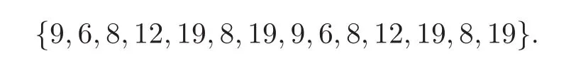

4.3 Different noise terms
5 Proof of Theorem 2.1


 Chinese Annals of Mathematics,Series B2018年4期