
Dynamic Analysis of High-Speed Boat Motion Simulator by a Novel 3-DoF Parallel Mechanism with Prismatic Actuators Based on Seakeeping Trial
2018-10-11 03:31:44AliPirouzfarJavadEnferadiMasoudDehghan
Ali Pirouzfar·Javad Enferadi·Masoud Dehghan
Abstract In this study,we focused on a novel parallel mechanism for utilizing the motion simulator of a high-speed boat(HSB).First,we expressed the real behavior of the HSB based on a seakeeping trial.For this purpose,we recorded the motion parameters of the HSB by gyroscope and accelerometer sensors,while using a special data acquisition technique.Additionally,a Chebychev highpassfilter was applied as a noise filter to the accelerometer sensor.Then,a novel 3 degrees of freedom(DoF)parallel mechanism(1T2R)with prismatic actuators is proposed and analyses were performed on its inverse kinematics,velocity,and acceleration.Finally,the inverse dynamic analysis is presented by the principle of virtual work,and the validation of the analytical equations was compared by the ADAMS simulation software package.Additionally,according to the recorded experimental data of the HSB,the feasibility of the proposed novel parallel mechanism motion simulator of the HSB,as well as the necessity of using of the washout filters,was explored.
Keywords Motionsimulators.Parallelmechanism.High-speedboat.Seakeepingtrial.Inversedynamics.Virtualwork
1 Introduction
In recent years,driving simulators have been widely used for educational and research purposes.With advancement in technology and decrease in cost,the advantages of using simulators for safe,economical,and environmentally friendly driving have become more apparent.The driving simulators’capability of producing a virtual driving environment can be used to train novice drivers before they are exposed to real world driving conditions.
Moreover,driving simulators are important in collecting data for environmental safety research,human factor studies,vehicle system development,and testing device development.These allow for the design,engineering,and ergonomics to bypass the design and development process of detailed vehicle interior mock-ups for human factor and vehicle performance studies(Utkan et al.2014;Chou and Fu 2007a,b).For this reason,the motion simulation of ships and other marine vehicles has always been of great interest to the naval architects.Throughout the course of human history,ships have played a significant role in traveling,trading,war,and military applications.The simulation of ship motions is an important topic of investigation in the education systems and entertainment industries.Ship motion simulation systems help trainee and game players in learning how to maneuver ships under different sea conditions.To design the requirements for the ship’s motion platform,some considerations must be made and should include the workspace based on head displacement envelope,payload,and load factor,kinematic parameters such as velocities and accelerations,and also a visual system to simulate some degrees of freedom(DoF)under certain conditions(Ueng et al.2008).
Subsequently,designing a proper mechanism to simulate the vehicle environment is one of the is sues that have attracted great attention of many researchers interested in simulator development.From this viewpoint,various different mechanisms can be proposed.Serial and parallel mechanisms are the two main mechanisms that have been utilized in precise manufacturing and medical science,as well as in various equipment and simulators.Patel and George compared these two mechanisms in their study(Patel and George 2012).They pointed out that,for certain applications,parallel mechanisms have several advantages over their serial counterparts.A parallel mechanism can be defined as a closed-loop kinematic chain mechanism,in which the end effector is linked to the base by several independent kinematic chains.Greater loadcarrying capacities (since total load can be shared by a number of parallel links connected to a fixed base),low inertia,higher structural stiffness,reduced sensitivity to certain errors,easy controlling,and built-in redundancy are some of their advantages.However,they have disadvantages such as smaller and less dexterous workspace due to the link interference, physical constraints of the universal and spherical joints,and actuator range of motion,in addition to suffering from platform singularities.Flint and Anderson carried out a study and concluded that the demand for higher accuracy and speed in large payload applications caused the recent trends toward the use of parallel mechanisms(Flint and Anderson 2001;Dongsu and Hongbin 2007;Teufel et al.2007).
Another approach toward classifying motion simulators and naval simulators is based on how they simulate the main 6-DoF.The ship motions consist of 6-DoF,i.e.,pitch,heave,roll,surge,sway,andyaw.These motions are divided into two categories.The first three movements are induced by sea waves,while the last three are caused by propellers,rudders,currents,and winds.Algorithms can be deduced to compute the magnitude of these motions based on Newton’s laws and other basic physical models of motion.Ship motion simulations are commonly designed to work with 3-or 6-DoF motion bases.Each system has advantages and disadvantages,which make them more suitable for specific applications.These two systems differ drastically when it comes to the cost of hardware,software,and complexity.Additionally,Larsen carried out a complete comparison of 3-and 6-DoF motion bases by utilizing classical washout algorithms(Chou and Fu 2007a,b;Larsen 2011).In conclusion,if the cost and design simplicity are important considerations,the 3-DoF system would be the best choice. However, 6-DoF motion base would be the best choice if full motion is required.
Dynamic analysis plays an important role in predicting the behavior of mechanical systems and achieving the best performance.There are two types of dynamic problems:(1)the direct dynamic problem of finding the manipulator’s response corresponding to the applied forces and/or torques and(2)the inverse dynamic problem of finding the actuator’s forces and torques required to generate the trajectory of the manipulator.There are three main methods to simulate dynamics equations,namely,the Newton-Euler laws,Lagrangian equations,and principle of virtual work.In the Newton-Euler method,it is necessary to write the equation of motion for each link.The inverse kinematics and dynamic analyses of the 6-UCU parallel mechanisms have been performed by the Newton-Euler method(Liu et al.2012).All the reaction forces and moments were eliminated during the dynamics analysis using the Lagrangian method.Staicu(2012)compared the inverse dynamic problem of the two known parallel mechanisms,namely,the spatial 3-PRS and planar 3-RRR,by means of the principle of virtual work,and verified them by Lagrange’s equations.Recently,many papers have been published based on the principle of virtual work.The generalized forces of a series-parallel mechanism have been determined by the screw theory and principle of virtual work(Garcia-Murillo et al.2013).The solution of the inverse dynamic problem of a 6-DoF parallel mechanism was performed by means of this principle and the concept of Jacobian matrices(Zhao and Gao 2009).Staicu presented recursive modeling in the dynamics of the Agile wrist spherical parallel mechanism by the principle of virtual work(Staicu 2009).Li introduced the inverse dynamics of a 3-PRC parallel mechanism(Li and Staicu2012).Tsai and Yuan(2010)solved the inverse dynamics of a 3-PRS parallel mechanism based on a special decomposition of reaction forces.Wang et al.(2010)formulated the inverse equations of the 2UPS2RPS by utilizing the virtual work principle.Almeida and Hess-Coelho(2010)introduced a dynamics model ofa 3-DoF asymmetric parallel mechanism and employed the virtual work principle by considering two assumptions,namely,lumped and distributed masses.In the above mentioned parallel mechanisms,U,C,R,P,and S stand for universal,cylindrical,revolute,prismatic,and spherical joints,respectively.
This paper proposes a special parallel mechanism class.This class is characterized by the addition of various passive segment constraints and is actually attracting great attention.This class of parallel mechanism reduces the number of solutions,which may be numerous in non-constrained parallel mechanisms,and causes difficulty in determining the solution of the geometrical model.The dynamical equations of motion were simplified and formulated by the principle of virtual work.Since the principle of virtual work is the most efficient method for the dynamic analysis of parallel mechanisms,it allows the elimination of joint constraint forces and moments from the motion equations.Moreover,one can derive the equations of motion in terms of a set of independent generalized coordinates.The addition of constraints also enables the determination of the orientation and position parameters or end-effector variables.This study aims to introduce a novel parallel mechanism for utilizing the motion simulator of an HSB.For this purpose,we used the experimental data of the HSB as the input parameters in the kinematic and dynamic analysis.
2 Description of HSB Motion System
The typical motion simulator can be divided into several components as follows:·Interior instruments of vehicle cabin·Visual and sound systems·Motion system·Control system
The simulation of inertial motion can be usually represented by the block scheme,as shown in Fig.1(Koekebakker 2001). The information originating from the simulated vehicle model cannot be directly applied to the platform in the form of motion commands. Since the motion platform has limited workspace, its boundaries would be quickly reached and the simulation of future motion cues would be prevented. The aim of the washout filters is to replicate the vehicle dynamics in the motion simulator, while keeping the platform within its boundaries (Correia Augusto and Loureiro 2009).
The proposed motion system for the HSB motion simulator is a 3(RPSP)-PU parallel mechanism. According to Fig. 2, this system consists of a mobile platform connected to a fixed platform via three active limbs and one passive central limb.Each of the three active limbs is made of revolute prismatic spherical prismatic(RPSP)joints,while the passive limb is made of prismatic universal(PU)joints.Therefore,the proposed manipulator has 11 links,which include the fixed link and13 kinematics pairs.The number of DoF for the 3(RPSP)-PU spherical parallel mechanism can be calculated by the Kutzbach-Grübler equation(Wampler 2006),as follows:where k is the number of links(k=12),n is the number of joints(n=14),λ is the degrees of the space within which the mechanism operates(λ=6),and fiis the DoF of the ith joint.By inspecting the entire manipulator,it can be seen that it has 3-DoF.

3 Seakeeping Trial
The seakeeping recording of the vessel is called the seakeeping trial,which is an important task performed for some vessels(Zeraatgar et al.2010).There is not a particular standard for the basis of ship seakeeping trial and researchers have used different methods according to their needs(Carrera and Rizzo 2005;Garme and Kuttenkeuler 2005;Jorgen et al.2005).Generally,to determine the ship motion model,such methods may include:
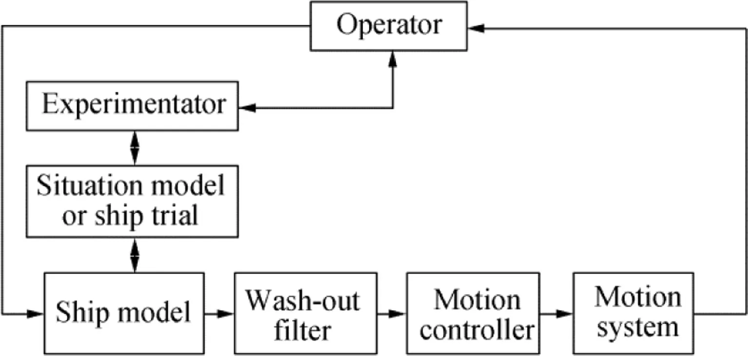
Fig.1 Block diagram of the general motion simulator
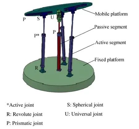
Fig.2 CAD model of proposed motion platform for HSB motion simulator
·Mathematical simulation of dynamic behavior
·Scale model testing
·Full-scale trial
We investigated the HSB model of the motion,during full-scale seakeeping trials conducted under a wide range of conditions(40 tests)in the Persian Gulf.As shown in Fig.3,a particular sea trial of the HSB was considered.For recording the HSB motions,we used various sensors such as GPS,gyro,and linear accelerometer,data logger,and laptop.These instruments are listed in Table 1,while the installed positions of these sensors on the HSB are shown in Fig.4.
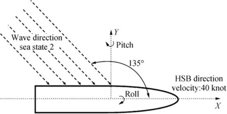
Fig.3 Particular HSB seakeeping trial
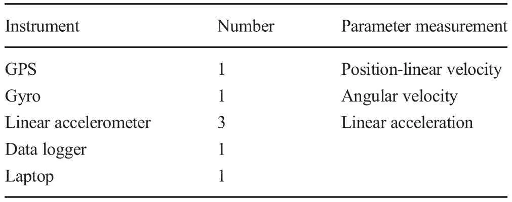
Table 1 Measuring instruments
Figure 5 shows the data recorded for the heave acceleration at the time of the particular sea trial,where the measurement was carried out by the A1 linear accelerometer.The heave acceleration data collected by the accelerator had two major problems.First,they made too much noise,and secondly,we observed that the diagram was ascending over time,while it should have been periodic.To overcome these problems,we used a high-pass filter to remove the unwanted low frequencies(which appeared to be increasing)and a low-pass filter to remove the high frequencies(which caused unwanted forces).Chebychev filters in the MATLAB software were used for frequency removal.Chebychev filters had higher precision than other classical filters and were more capable of eliminating the interfering signals.The frequency range of the HSB movements along the z axis was approximately 0.5-5 Hz.Therefore,frequencies more than 5 Hz were eliminated by a low-pass filter,while the frequencies below 0.5 Hz were eliminated by a high-pass filter.In comparison to other classical filters,the Chebyshev filter had higher accuracy and greater ability in eliminating the disturbing signals.The order of the filter represented the curve slope in the response graph of the filtering frequency.When the filtering frequency increased,the damping of the frequency response curve became higher,especially after the cutoff frequency(for the low-pass filter)and before the cutoff frequency(for the high-pass filter).Consequently,the precision increased.It is certain that if the filter order increased,its implementation would become more complex due to the addition of the active element in the electrical circuit(e.g.,inductor and capacitor).Due to the simple implementation of second-order filters and their additional damping characteristics in comparison to the first-order filters,the second-order filters are generally used in such applications.Therefore,to eliminate the disturbing frequencies above 5 Hz and lower than 0.5 Hz,the low-pass and high-pass Chebyshev filters of the second order were used in the MATLAB software.The function block parameters of the second-order Chebyshev filter that were used in the MATLAB software are presented in “Appendix”.The motion parameters are shown in Figs.6,7,and 8,after integration and filtering.
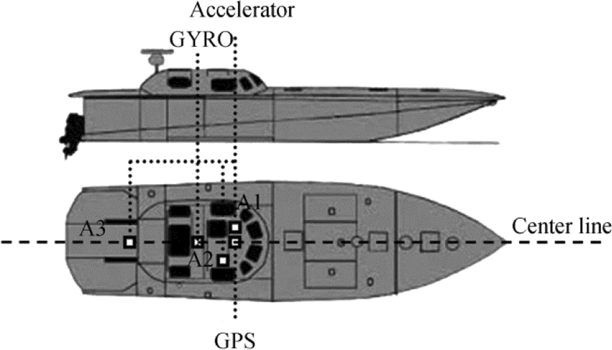
Fig.4 Schematic of HSB and installed positions of sensors
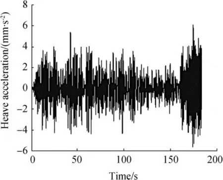
Fig.5 Heave acceleration of HSB
Figures 9 and 10 show the data recorded by the gyro sensor.This gyro was installed exactly under the pilot’s chair,as shown in Fig.4.
Since the output of the gyro consisted of the filtered data,we could use this data directly for integration.Then,the angular velocity of the HSB, roll and pitch time rate, and angular position of the HSB could be readily obtained. These parameters are shown in Figs. 11, 12, 13, and 14 and are depicted in the range of 0-10 s to obtain a clearer view. According to these figures, the parallel mechanism that could simulate all the motions of the HSB should have the following features:
· Maximum roll angle±15°
· Maximum pitch angle±15°
· Maximum heave position equal to±250 mm
We use the heave position,roll,and pitch angles for simulating the motion of the HSB in the dynamics analysis.
4 Description of Motion Platform Kinematics Parameters
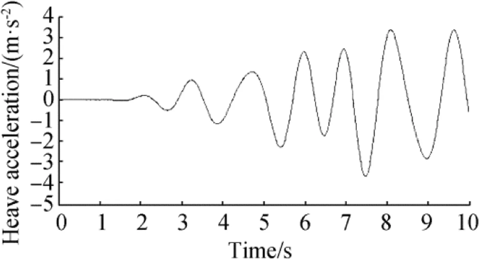
Fig.6 Filtered heave acceleration
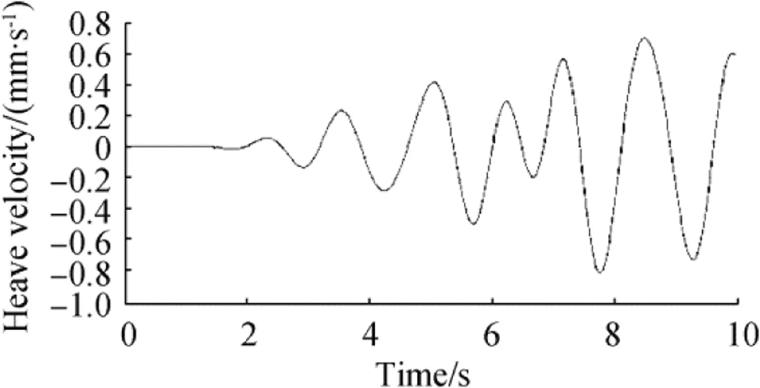
Fig.7 Filtered heave velocity
In this section,we define all the required parameters for the kinematics analysis of the proposed motion platform.These parameters consist of unit vectors,scalar parameters,and rotation matrices,as shown in Fig.15.The rotation axis of the angular joint is defined along the unit vector ui.The angle θidefines the rotation value of the actuated joint about the unit vector uiby the right thumb rule.The variable distance of the universal joint on the passive central limb from the center of the base platform O is denoted by vector h.The unit vector eiis defined along AiDi.The prismatic joint slides along the unit vector ei.Each limb consists of two parts,namely,the lower link(cylinder)and upper link(rod).The spherical joint is located at the end of the upper link.The unit vector viis defined along the vector Ssi.The center of the spherical joint is at the intersection of the axes of the unit vector eiand unit vector vi.The variable length of each actuated limb is denoted byli.The upper prismatic joint slides along the axis of the unit vector vi.The variable distance of the upper prismatic joint from the fixed spherical joint SDiis denoted by bi.Moreover,it was assumed that all the viunit vectors existed on a plane.Furthermore,the fixed distance of the revolute joint from the center of the base platform O is denoted by ai.
The description of the coordinate frames was required for the inverse kinematics analysis,velocity analysis,acceleration analysis,virtual displacements,and dynamic analysis of the motion simulator.For these analyses,we defined the coordinate frames as shown in Fig.15.
·The fixed coordinate frame{B}was located on the center of the fixed platform.The xBaxis of this frame was along the unit vector u1.The zBaxis was defined along ui×ui+1.The yBaxis was specified by the right hand rule.
·The moving coordinate frame{M}was attached to the moving platform,whose origin coincided with the universal joint of the passive central limb.The xMaxis of this frame was along the unit vector v1.The zMaxis of this frame was along the direction perpendicular to the moving platform in the direction of vi×vi+1.The axis yMwas specified by the right hand rule.
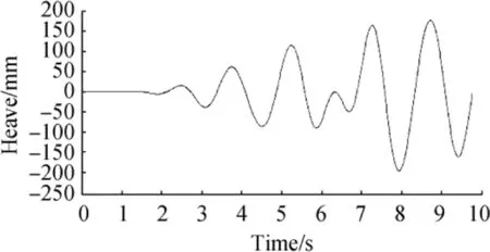
Fig.8 Filtered heave position
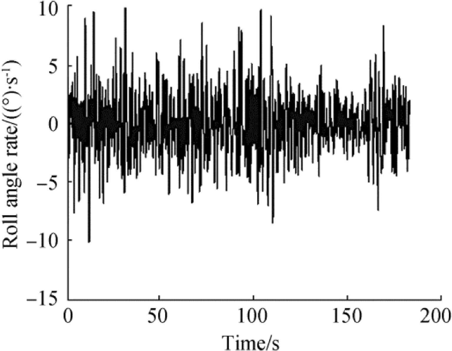
Fig.9 Roll angle rate of HSB
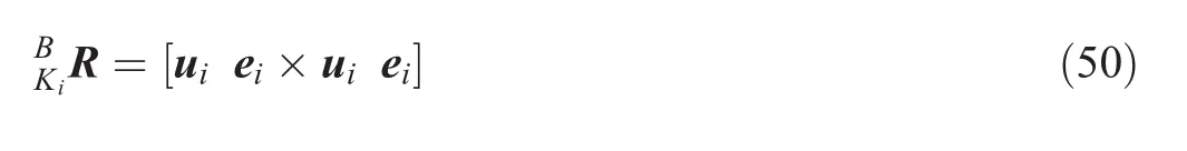
·The coordinates frame{Ki}was attached to the lower link,whose origin was on the revolute joint.The xKiand zKiaxes of this frame were along the unit vector uiand unit vector ei,respectively.The yKiaxis was also specified by the right hand rule.
5 Inverse Kinematics Analysis
Kinematics is the science of motion that treats motions without regarding the forces causing it.In the inverse kinematics problem,the position and orientation of the mobile platform of the manipulator are given and are calculated all possible sets of joint angles that could be used to attain this given position and orientation.A solution of the inverse kinematics problem is required for velocity,acceleration,and dynamics analysis.For this purpose,the orientation of the mobile platform with respect to the fixed platform is known.As shown in Fig.15,this mechanism consists of three kinematic chains.Therefore,for each kinematic chain,we can write the following relation:
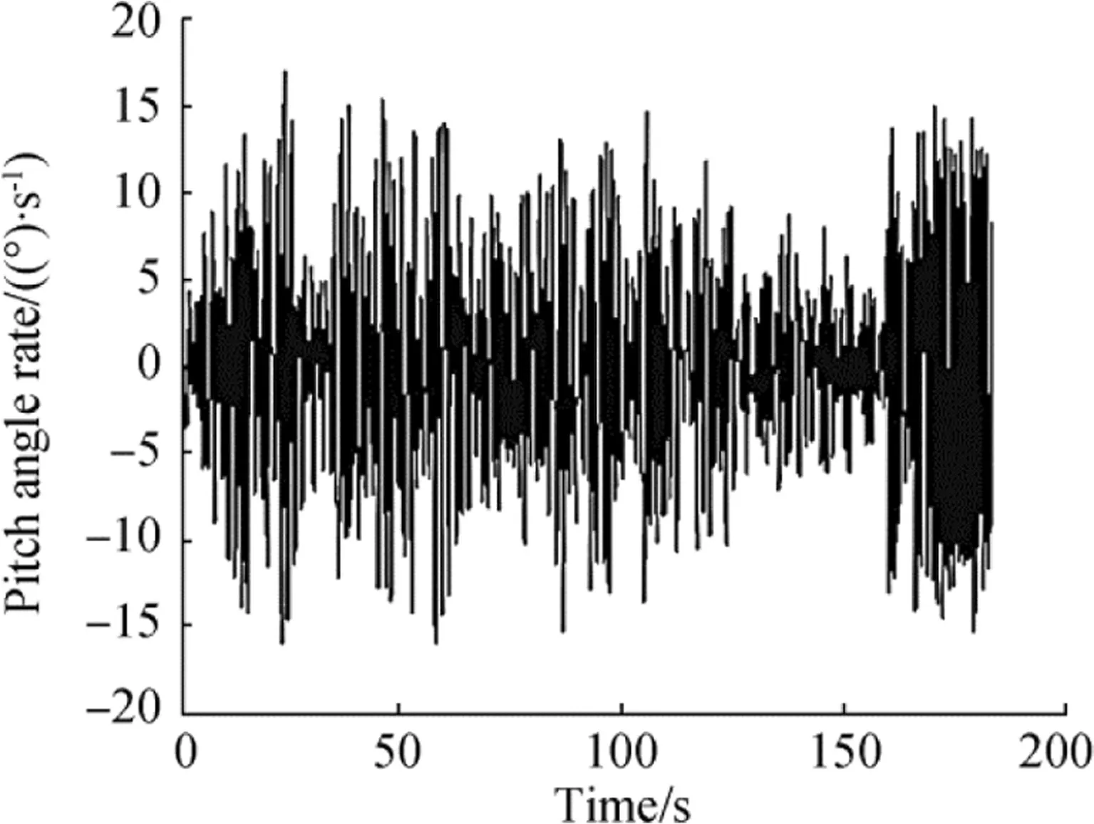
Fig.10 Pitch angle rate of HSB
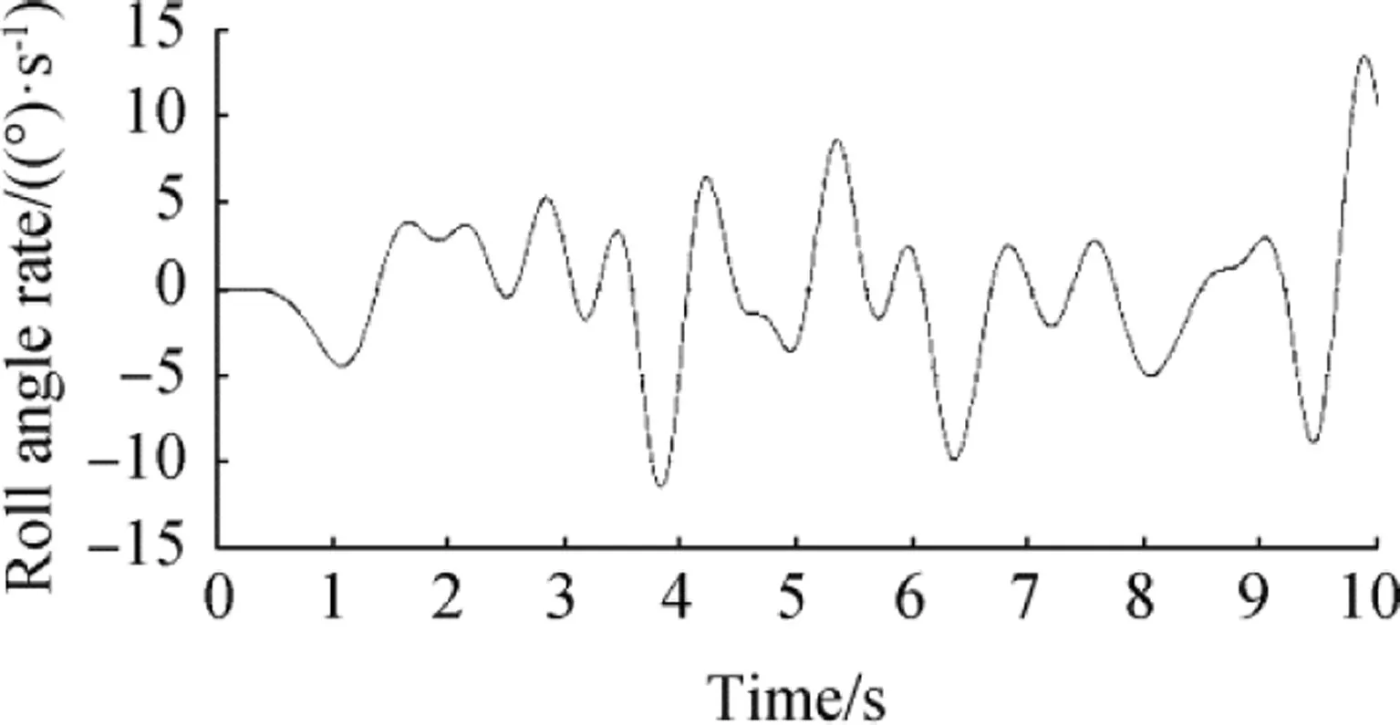
Fig.11 Filtered roll angle rate

where
Additionally,the relationship between the unit vector viin the fixed coordinate frame and the moving coordinate frame can be written as:

whereMviis described in the moving coordinate frame as:
Therefore,we can rewrite Eq.(2)as follows:

To obtain length li,we can multiply both sides ofEq.(4)by

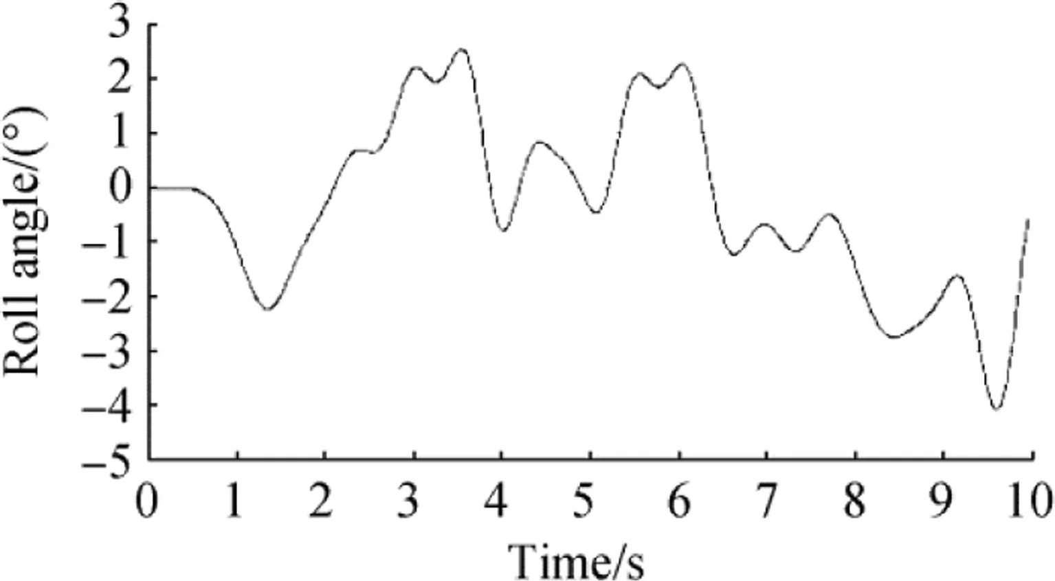
Fig.12 Filtered roll angle
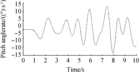
Fig.13 Filtered pitch angle rate

Next,the length liof each leg is computed as follows:

Finally,the direction of each leg can be obtained as follows:

If the unit vector k rotates about the unit vector uiin the positive direction by angle θi,the direction of each leg can be obtained by Rodrigues’rotation formula(Wampler 2006)as follows:
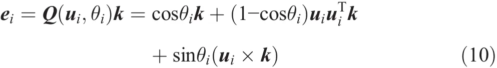
where k=[0 0 1]T.The unit vector uiis perpendicular to the unit vector k;therefore,the above equation can be simplified as follows:
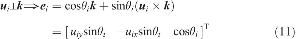
where uixand uiyare the Cartesian components of the unit vector uiin the base coordinate frame.Finally,the closed form solution of the inverse kinematics problems is given by:
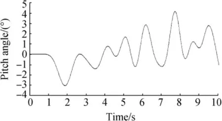
Fig.14 Filtered pitch angle
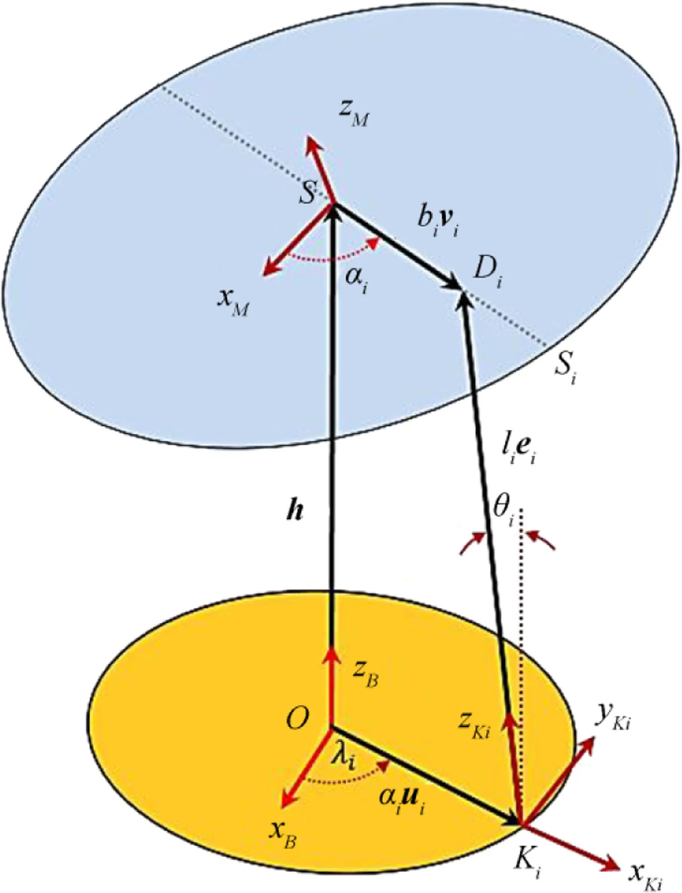
Fig.15 Coordinate frames and parameters of the ith kinematics chain
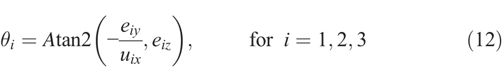
where eix,eiy,and eizare the components of the unit vector eiin the base coordinate frame.As shown in the above equation,the inverse kinematics problem of the manipulator has a unique solution.
6 Inverse Velocity Formulation
6.1 Limb Velocity Analysis
In this subsection,we obtain the relation between the motion of the moving platform and the motion of all passive and active joints.These relationships will be used when solving the inverse dynamics problem by utilizing the virtual work method.
By using the time derivative of Eq.(2),the velocity of each leg can be written as:


To find the relationship for˙li,the term of[vi× (ui× ei)]Tmust be multiplied on both sides of the above equation;therefore,we have:

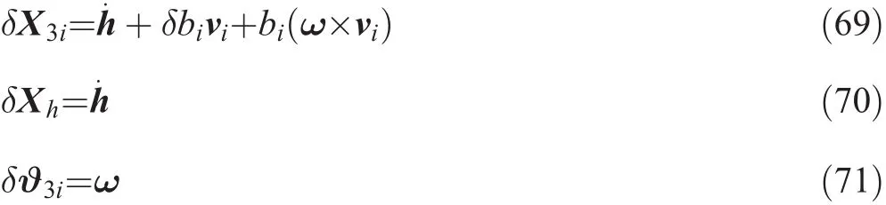
To obtain the time rate of the prismatic passive joint on the moving platform b˙i,we first multiply the term uiTon both sides of Eq.(14)as follows:


where
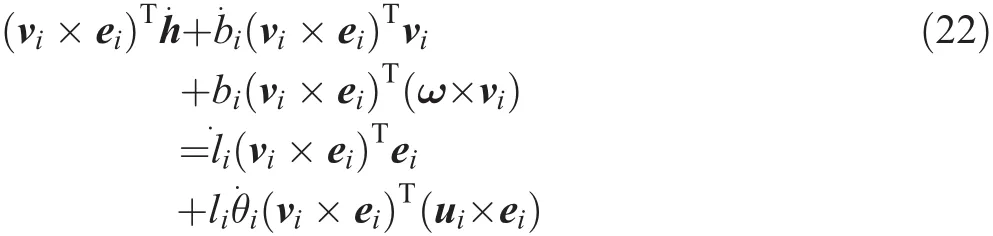
Since(vi× ei)Tvi=(vi× ei)Tei=0,Eq.(22)can be simplified as follows:
where
6.2 Input and Output Velocity Analysis
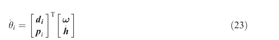
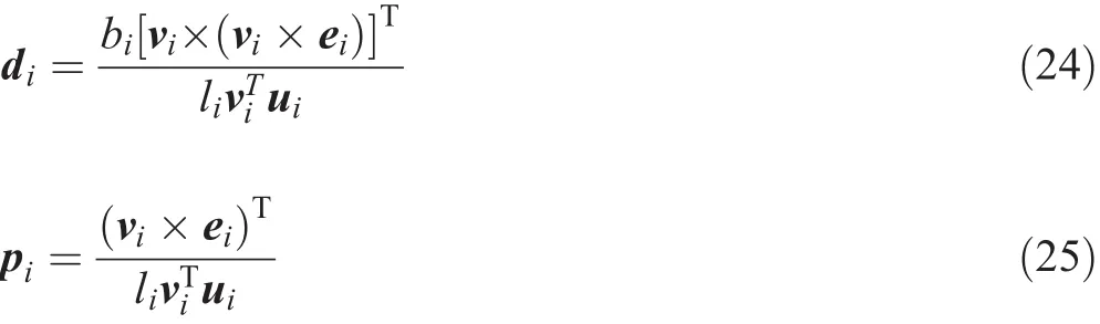
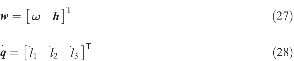
The relationship between the twist vector of the moving platform w and the position rate of the actuators q˙,in the parallel mechanism,is expressed by a Jacobian matrix as follows:

where J and K are two Jacobian matrices of the manipulator at hand and
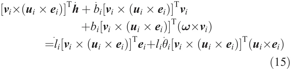
The main equation specifying the velocity relationships of each kinematics chain is written by Eq.(15),by using the vector triple product,as follows:
Therefore,Eq.(15)can be simplified as follows:

The above equation for i=1,2,and 3 can be assembled and expressed in vector form;therefore,we can define J and K as follows:

7 Acceleration Analysis of Limbs
In this section,we obtain the relation between the angular velocity and angular acceleration of the moving platform,and the value of the acceleration of all passive and active joints.These relationships will be used while solving the inverse dynamics problem.
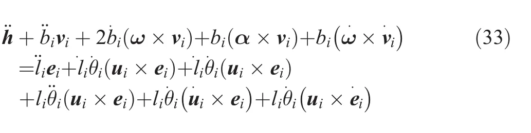
The acceleration of each term is obtained by taking the time derivative of Eq.(14);therefore,the acceleration of each link can be written as follows:
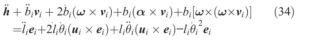
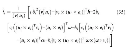
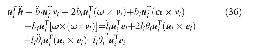
By multiplying both sides of the above equation by[vi×(ui×ei)]Tand simplifying,we obtain¨lias a function of¨h,ω,and α,as follows:

Similarly,we can obtain the scalar valueby multiplying(vi×ei)Ton both sides of Eq.(34)and simplifying as follows:
8 Dynamics Modeling
By inverse dynamics,the required joint actuator torques/forces were computed from the specification of the robot’s trajectory(position,velocity,and acceleration).For a rigid robot,the inverse dynamics is a straightforward algebraic computation obtained by replacing the desired motion of the generalized coordinates in the dynamic model.The minimum requirement for the exact reproduction is that the planned motion must have a continuously differentiable desired velocity.By knowing the pose and kinematic state of each link as well as the external forces acting on the robot, the torque of the actuators,or the active forces required by a given motion of the moving platform,can be formulated based on three main methods that may be utilized to compute the actuated torques.The first one is to use the classical Newton-Euler procedure,the second one uses Lagrange’s equations,and the third one is based on the principle of virtual work.
Unlike serial manipulators,parallel mechanisms always contain passive joints.Among these methods,virtual work allows the elimination of constraint forces and moments at the passive joints,from the motion equations.Therefore,the virtual work method can offer certain advantages.The principle of virtual work states that a mechanism is under dynamic equilibrium if and only if the virtual work developed by all external,internal,and inertia forces vanishes during any virtual displacement compatible with the kinematics constraints.In this section,the dynamical equations of motion are formulated by using the principle of virtual work.In this paper,for simplicity,we will assume that the frictional forces at the joints are negligible.The equation of motion by the principle of virtual work for the manipulator can be written as follows:
where δq and δXpare the virtual displacement vectors of the actuators and the moving platform in the base and the moving coordinate frames,respectively.Additionally,andKare the virtual displacement vectors of each body in the active links with respect to the coordinate frame attached to them,whileBis the virtual displacement vector of the body in the passive link.
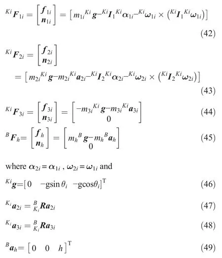
8.1 Applied Forces:Torques and Inertia
We consider that the(6×1)vector of the generalized forces acting on the moving platform is expressed as follows:
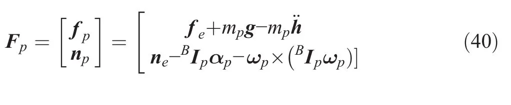
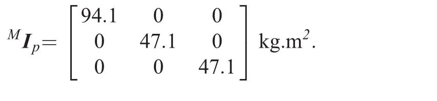
where fpand npare the resultant forces and resultant moments,respectively.Additionally,feand neare the external forces and moments exerted at the mass center of the moving platform,respectively,and Ipis the inertia matrix of the moving platform with respect to the base coordinate frame{B}.
whereMIpis the inertia matrix of the moving platform with respect to the moving coordinate frame,{M}.
The vectors of the generalized forces applied to the mass center of each body in the active and passive links with respect to the link coordinate frame{Ki},can be expressed as follows:
8.2 Virtual Displacement
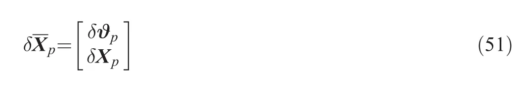
A virtual displacement is an assumed infinitesimal change in a system coordinate occurring while time is held constant.Since no actual displacement occurs without the passage of time,it is called virtual rather than real.Therefore,we define the virtual displacement of the moving platform as follows:
Additionally,by the Jacobian matrices in Eq.(26),we can obtain the virtual displacement of the active joints versus the virtual displacement of the moving platform as follows:

where Jp=-J-1K.Now,to determine the virtual displacement of the active and passive links,as the first step,we obtain the mass center position vector of the links(see Figs.15 and 16)as follows:
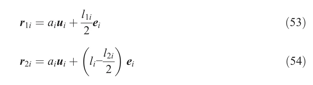
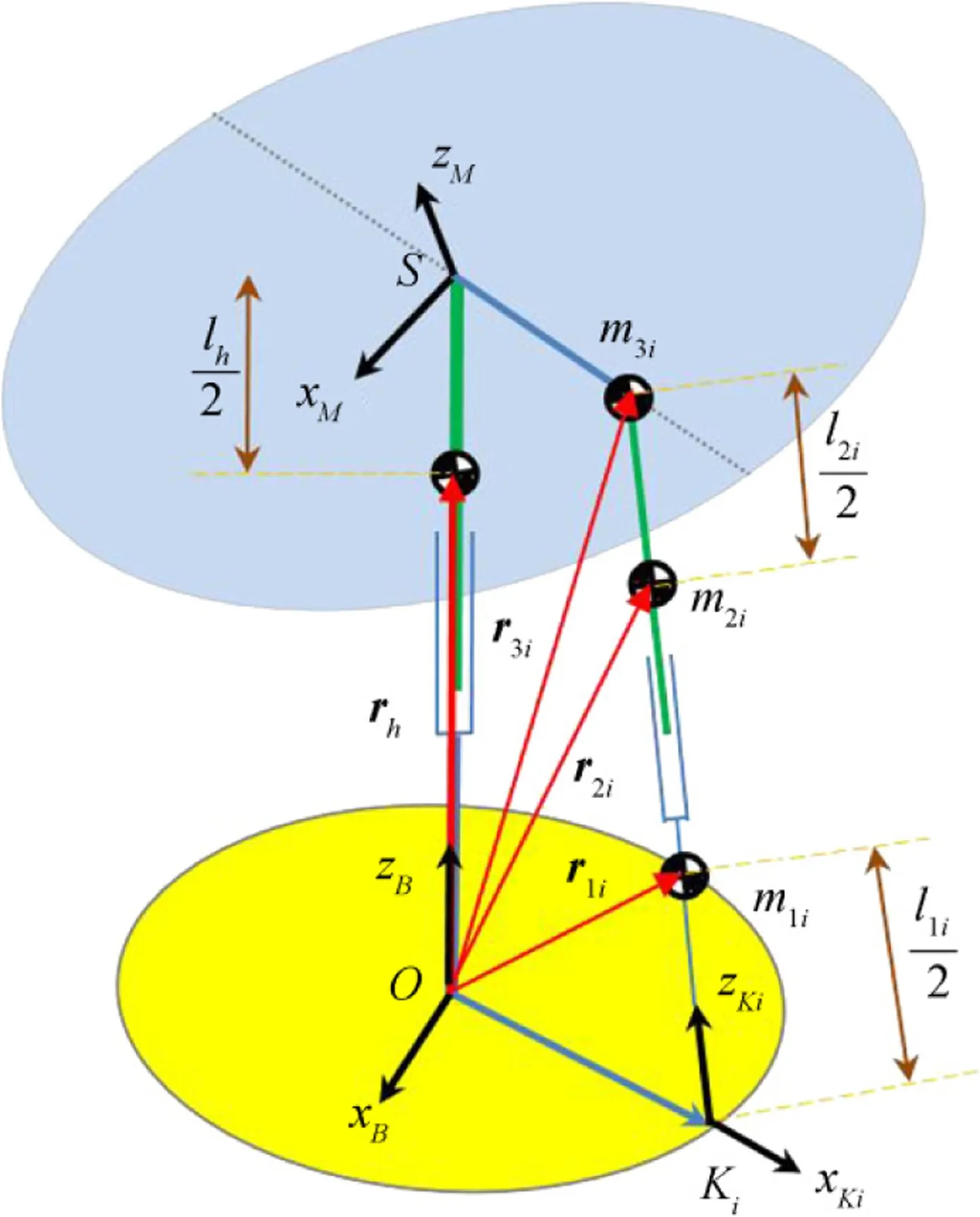
Fig.16 Mass centers and their positions
Additionally,we know that the angular velocity of bodies1 and 2 in the ith active link is as follows:

Therefore,the virtual displacement of the bodies can be obtained as follows:
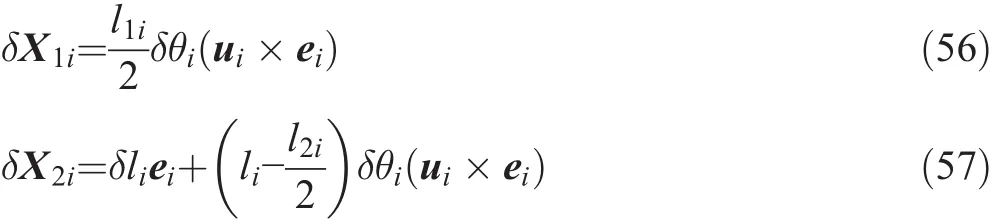
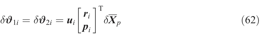
whereδϑ1i=δϑ2i=δθiui.Additionally,by using Eqs.(16)and(23),we can write:
Therefore,substituting the above equations in Eqs.(56)and(57)leads to:
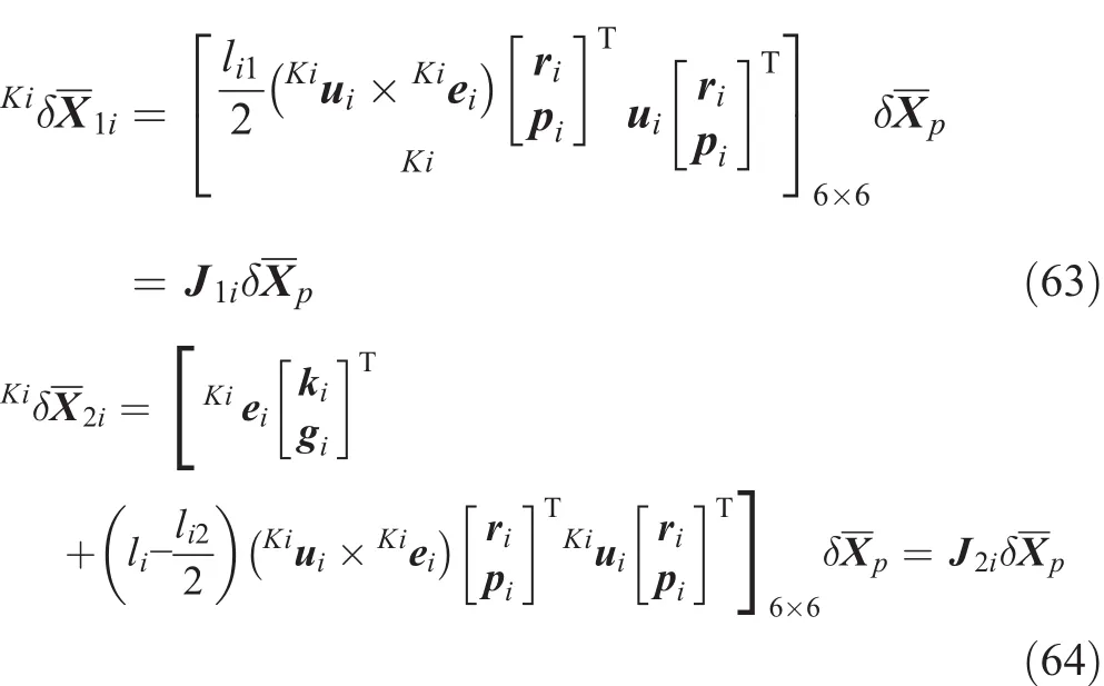
Similarly,we can write:
Therefore,the general virtual displacements of each body in the active links in the coordinate frame{Ki}are as follows:
According to Figs.15 and 16,the position vector of the passive links’mass center can be written as follows:

And we know that:
Additionally,the virtual displacement of each body in the passive links can be written as follows:
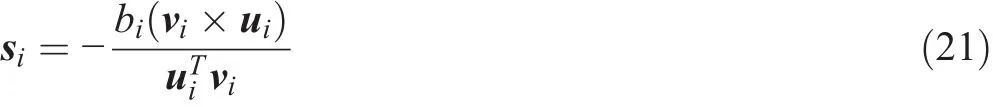
Additionally,by Eq.(20),we can write:

Now,we can substitute the above equation into Eq.(69)and obtain:
where Viis an axisymmetric matrix consisting of the components of vector viin the base coordinate frame,as follows:
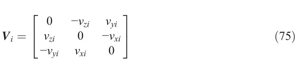
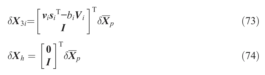
Therefore,in terms of the virtual displacements of the moving platform in the coordinate frame{Ki},the virtual displacements of each body in the passive links can be written as follows:
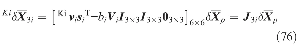
Finally,we can write the virtual displacement of the bodies in the coordinate frame{B}as follows:
whereKiui=[1 0 0]T,Kivi=[0 1 0]T,andKiei=[0 0 1]T
8.3 Dynamic Equations of Motion
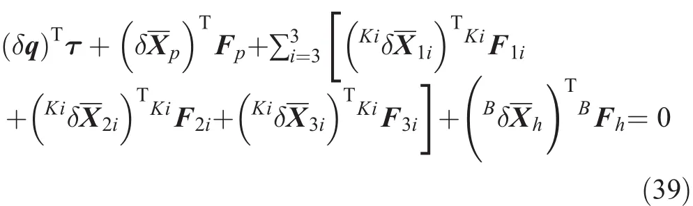
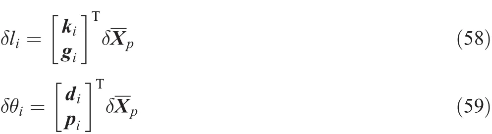
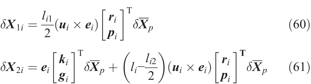
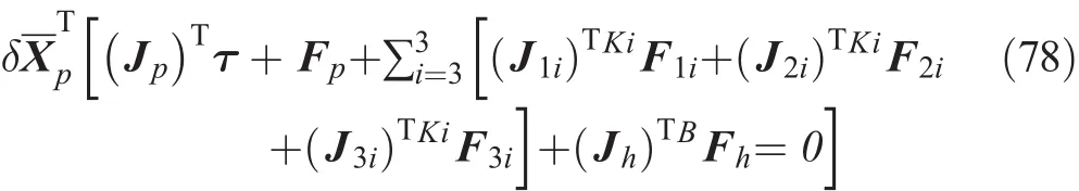
The virtual displacements in the equation of motion(61)must be compatible with the kinematic constraints imposed by both active and passive joints.Therefore,it is necessary to relate the above virtual displacements to a set of independent generalized virtual displacement.Therefore,we can substitute Eqs.(40),(42),(43),(44),(45),(52),(63),(64),(76),and(77)in to the main equation of the virtual work,i.e.,Eq.(39),and thereby we can write:
Since the above equation is valid for any δXp,it follows that:
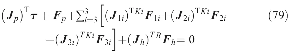
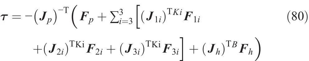
Equation(79)provides the dynamic equations of the 3RPSP-PU manipulator.This equation shows that the dynamics of this manipulator can be reduced to solving a system of linear equations with three unknown force actuators.Therefore,we can obtain the input forces required to produce the desired trajectory of the moving platform as follows:
9 Numerical Example
As described in the preceding sections,a computer program was developed by the MATLAB software and forces required to generate the desired trajectories were eventually obtained.To verify this methodology,three case studies were considered and the required forces were compared by using a dynamics modeling commercial software(ADAMS).Finally,as shown in Figs.5,6,and7,the motions of the HSB in the seakeeping trial of the moving platform were supplied and the required forces were calculated.
9.1 Manipulator Specifications
Note that the dimensions and mass properties of the manipulator were picked up based on the approximate dimensions and mass properties of the HSB cabin simulator.
(a)Architecture parameters
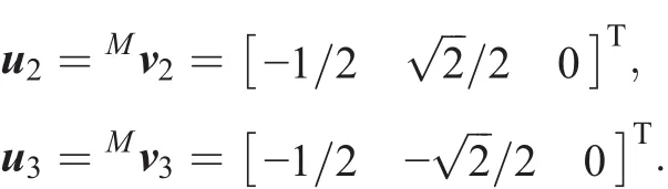
Let us assume that ai=0.3m,l1i=l2i=0.3m,α1=λ1=0°,α2= λ2=120°,and α3= λ3=240°.Therefore,we can write:u1=Mv1=[1 0 0]T;
(b)Mass properties of the moving platform
ms=1176 kg
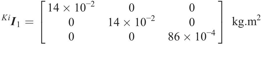
(c)Mass properties for each lower link,i=1,2,3
m1i=17 kg
(d)Mass properties for each upper link,i=1,2,3
(e)Mass properties for each upper prismatic link,i=1,2,3
m3i=3 kg
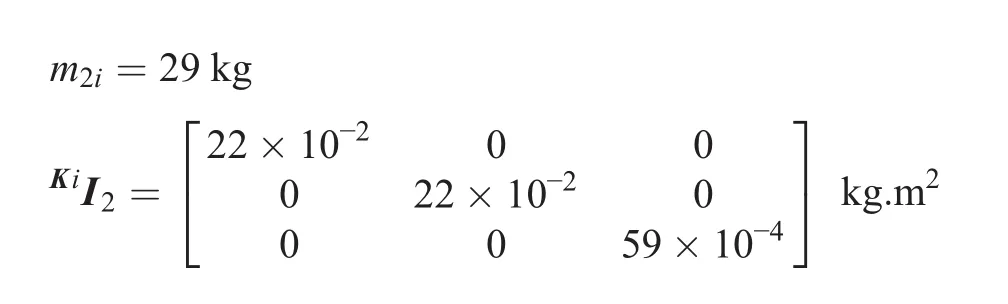
(f)Mass properties for the passive central limb
m3i=29 kg
9.2 Trajectory of Moving Platform
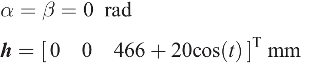
9.2.1 Vertical Motion
To confirm the obtained dynamic equations,we assumed that the moving platform had only vertical motion and no rotational motion.In this case,we expected that the forces producing this trajectory and the force required by the actuators are equal.Therefore,we assumed that this trajectory was as follows:
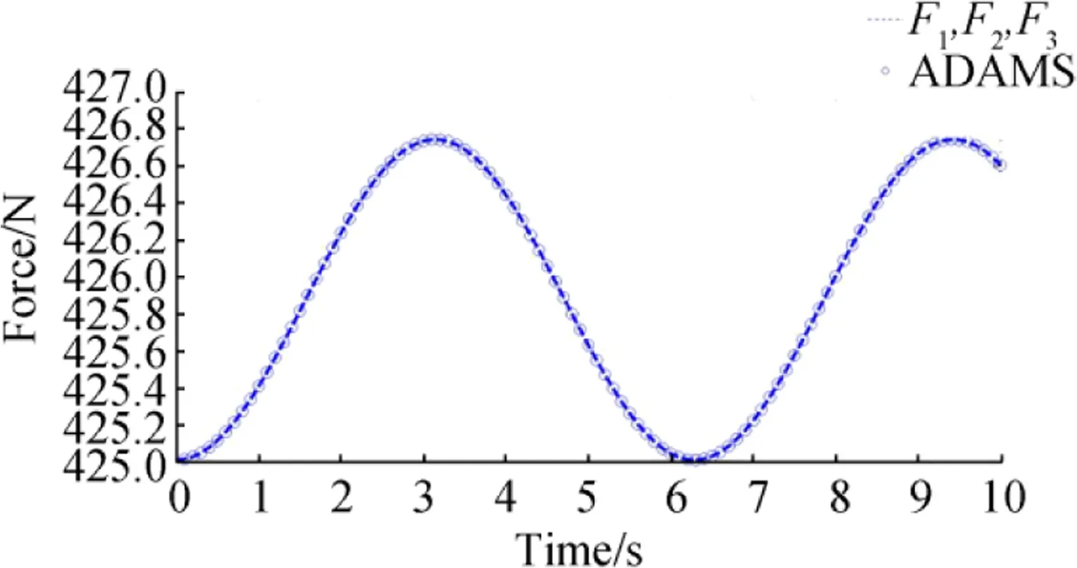
Fig.17 Comparison of analytical model and ADAMS for vertical motion
By referring to the methods described in the previous sections,the required forces were calculated as a function of time.As expected,the values of the three motor torques remained equal during the simulation.To further verify our analytical model,the trajectory was simulated by using a dynamic modeling commercial software.The results of this simulation and our analytical model were plotted and are shown in Fig.17.As the two results were indistinguishable,these results verified the correctness of our analytical model.Additionally,based on the fact that only the vertical motion was defined in this movement,it would be reasonable if the force of the three arms was the same. On the other hand, due to the cosine motion of the moving platform,it was clear that the force applied to the arms should also be applied to the cosine forms.
9.2.2 Rotational Motion
In this trajectory, the rotational motion of the moving platform was at a constant height.In this case,the trajectory of the moving platform could be given by:
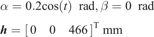
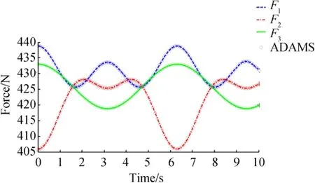
Fig.18 Comparison of analytical model and ADAMS for rotational motion
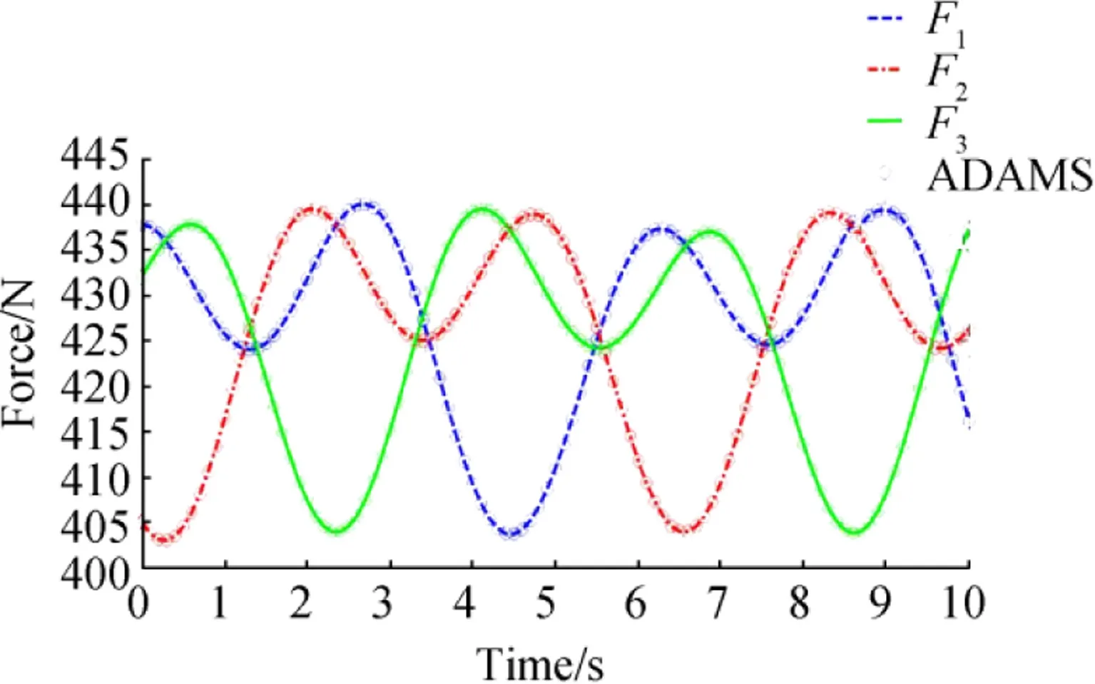
Fig.19 Comparison of analytical model and ADAMS for first general motion
The three forces were calculated as functions of time.Additionally,this trajectory was simulated by using the ADAMS software.The results of these simulations and the analytical model were plotted and are shown in Fig.18.These results also verified the correctness of our analytical model.
9.2.3 General Motions
(a)In this trajectory,the moving platform had two rotational and vertical motions.The trajectory of the moving platform was specified as follows:
The results of this trajectory are presented in Fig.19.Since the two results(ADAMS and analytical model)were indistinguishable,they verified the correctness of the analytical model.
(b)In this trajectory,the moving platform had a rotational motion around the Y axis and a transition movement along the Z axis.The trajectory of the moving platform was specified as follows:


Fig.20 Comparison of analytical model and ADAMS for second general motion
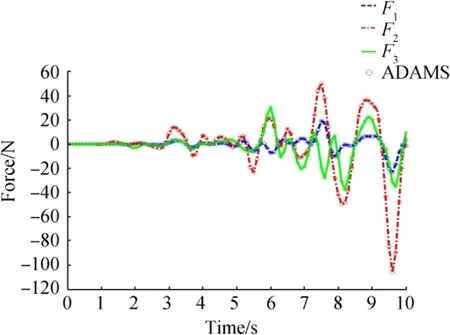
Fig.21 Comparison of analytical model and ADAMS for HSB simulator at seakeeping trial
The results of this trajectory are presented in Fig.20.The matching analytical model and ADAMS results verified the correctness of the analytical model.
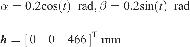
9.2.4 Experimental Trajectory of HSB at Seakeeping Trial
In this simulation,the trajectory of the moving platform was assumed as shown in Figs.5,6,and 7 of the HSB in seakeeping.The input forces were calculated,plotted,and shown in Fig.21.The matching analytical model and ADAMS results also verified the correctness of the analytical model.
1 0 Conclusions
In this study,a novel parallel mechanism for the motion simulator of a HSB was proposed.Additionally,we measured the real behavior of the HSB based on the seakeeping trial by a special data acquisition technique and a gyroscope.We used a Chebychev high-pass filter to eliminate the noise in the accelerometer sensor.Then,the problem of the manipulator’s inverse kinematics was solved and a methodology for solving the inverse dynamics of the manipulator was developed by using the inverse velocity and inverse acceleration analysis.The constraint forces were eliminated at the outset using the principle of virtual work.This allowed us to reduce the inverse dynamics of the manipulator to solve a system of three linear equations.To verify the methodology,three case studies were presented,and it was demonstrated that this methodology had good accuracy.Finally,the required forces for the HSB simulator were calculated.The high accuracy and validity of the kinematic and dynamic equations were observed with regard to the comparison of the analytical equation outputs and the ADAMS simulation software(identical graphs),which were investigated with several different samples.
Appendix
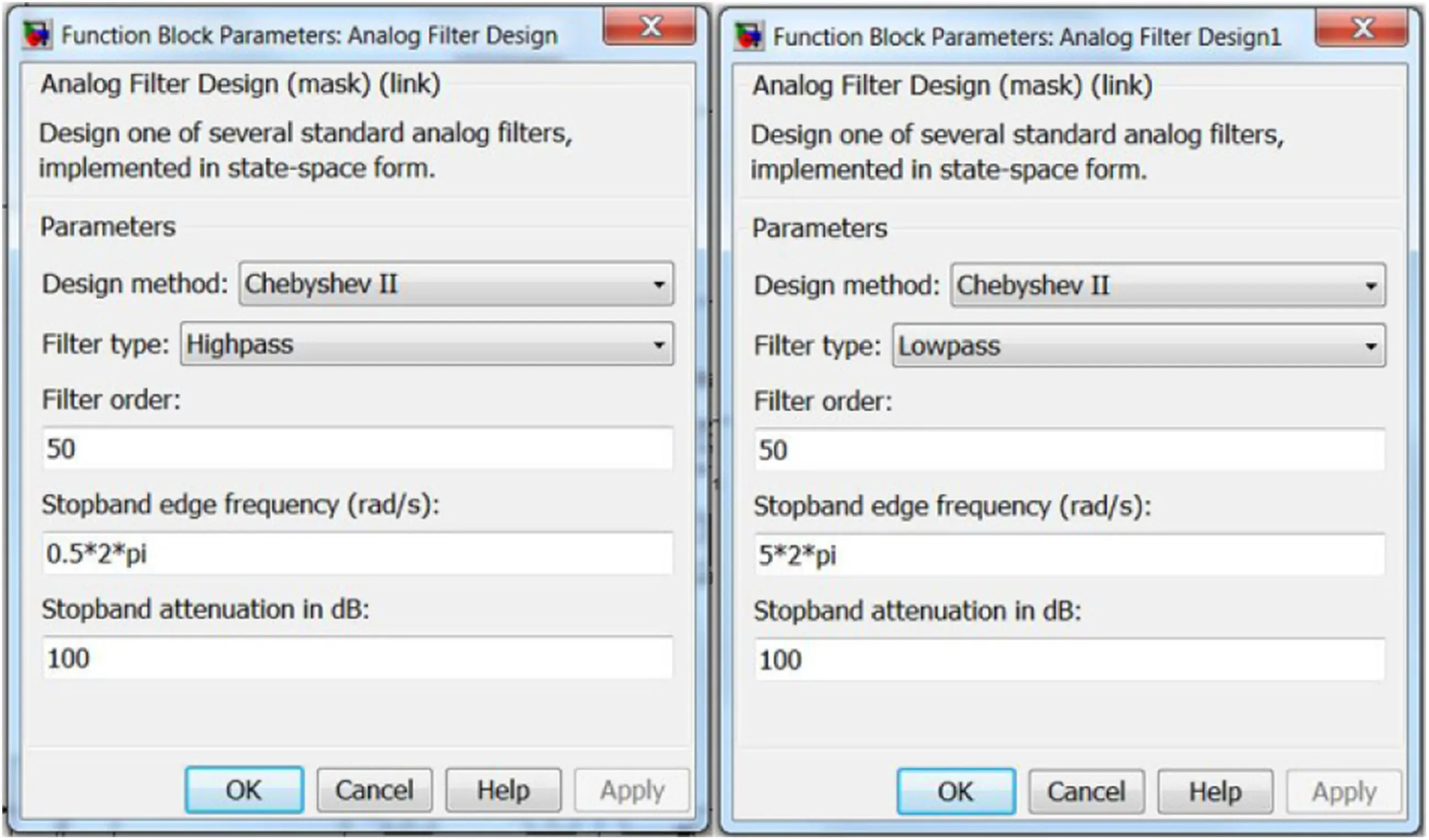
Fig.A1 The function block parameters of the second-order Chebyshev filter used in the MATLAB software
 Journal of Marine Science and Application2018年2期
- Journal of Marine Science and Application的其它文章
- Fast Ferry Smoothing Motion via Intelligent PD Controller
- Internal Resonances for the Heave Roll and Pitch Modes of a Spar Platform Considering Wave and Vortex Exciting Loads in Heave Main Resonance
- Comparison of Scour and Flow Characteristics Around Circular and Oblong Bridge Piers in Seepage Affected Alluvial Channels
- Empirical Equilibrium Beach Profiles Along the Eastern Tombolo of Giens
- Determining the Scour Dimensions Around Submerged Vanes in a 180°Bend with the Gene Expression Programming Technique
- Structural Design and Performance Analysis of a Deep-Water Ball Joint Seal