Quantifying growth and breakage of agglomerates in fluid-particle flow using discrete particle method☆

Lingfeng Zhou ,Junwu Wang *,Wei Ge ,Shiwen Liu ,Jianhua Chen Ji Xu Limin Wang Feiguo Chen Ning Yang Rongtao Zhou ,Lin Zhang Qi Chang ,Philippe Ricoux ,Alvaro Fernandez

1 State Key Laboratory of Multiphase Complex Systems,Institute of Process Engineering,Chinese Academy of Sciences,Beijing 100190,China

2 University of Chinese Academy of Sciences,Beijing 100049,China

3 Tianjin University,Tianjin 300072,China

4 TOTAL SA-R&D Groupe,Paris 92069,France

5 Total Research&Technology Feluy,Belgium,Germany

1.Introduction

Fluid-particle flows featuring spatio-temporal multi-scale structures are typically complex systems,in which particle aggregation is a common phenomenon[1,2].When the cohesive force between the particles is small enough to be ignored,particle aggregations exist in the form of clusters[3].However,cohesive particles gather to form agglomerates,which are more compact and stable than clusters[4].To some extent,the agglomerates hinder the mass and heat transfer between the fluid and the particles[5-7].In industry,a great number of problems appear due to the agglomerates.For example,the occurrence of agglomerates during the production of polyethylene can lead to defluidization[8].Therefore,it is necessary to investigate the characteristics and mechanism of agglomeration.

At present,agglomerates can be characterized by experiment,theoretical analysis and simulation.The experiment not only can observe the morphology of the agglomerates directly,using such as the optical fiber probe technology[9]and high speed imaging technology[10],but also can relate the characteristics of agglomerates to pressure drop signals and acoustic wave,such as pressure fluctuation method[11]and acoustic emission method[12].However,it is very difficult to get all information of the flow and particles to reveal the essential mechanism of agglomeration.Theoretical analysis is often based on the global balance of force[13]or of energy[14,15]to establish a model to predict the size of agglomerates.In view of the weakness of experimental and theoretical quantification,many scholars have used particle-scale simulation methods to investigate the agglomerates,and the effects of particle properties, fluid properties,types of cohesive forces and operation conditions on the agglomerates have been explored[16-19].However,the quantitative advantages of simulation as well as the mechanism of agglomeration are not fully explored yet.

In this paper,a solid-liquid flow system including millions of cohesive particles is simulated by the discrete particle method(DPM)[20].Taking full advantage of DPM to track the location and velocity of any particle at any moment,therefore,the state of particles entering or leaving agglomerates can be tracked,the growth and breakage process of all agglomerates can also be monitored quantitatively.A method is then proposed to quantify the growth and breakage of agglomerates.It was found that the growth rate and breakage rate are functions of the size of the agglomerates,and an equilibrium point between the growth and breakage of the agglomerates exists at a certain size of the agglomerates,which is consistent with the most probable size of the agglomerates.

2.Discrete Particle Method

In recent years,computer simulation develops rapidly and becomes a powerful tool for the research of fluid-particle systems,among which DPM is a typical method characterized by the disparity of the resolutions of description for the particles and the fluid[21-23]:the solid particles are tracked individually and the fluid flow is computed at a scale much larger than the particles.The liquid phase is hence described by the volume-averaged Navier-Stokes equations[22],

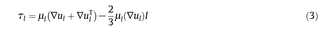
where τlis the stress tensor,which is calculated as

The discrete element method(DEM[24])is usually employed for tracking the particles,where the equation for the motion of a particle is

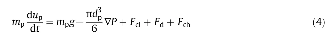
The five items on the right hand side of the equation are gravitational force,pressure gradient force,collision force,drag force and cohesive force,respectively.The collisional force between particle-particle or particle-wall collisions(Fcl) is calculated using the linear spring and dashpot model[24],which is calculated as follows:

wherekis the elastic constant,δnis the overlap of two particles,γ is the viscoelastic damping constant,vijis the normal component of the relative velocity of two particles.kand γ are calculated as follows:

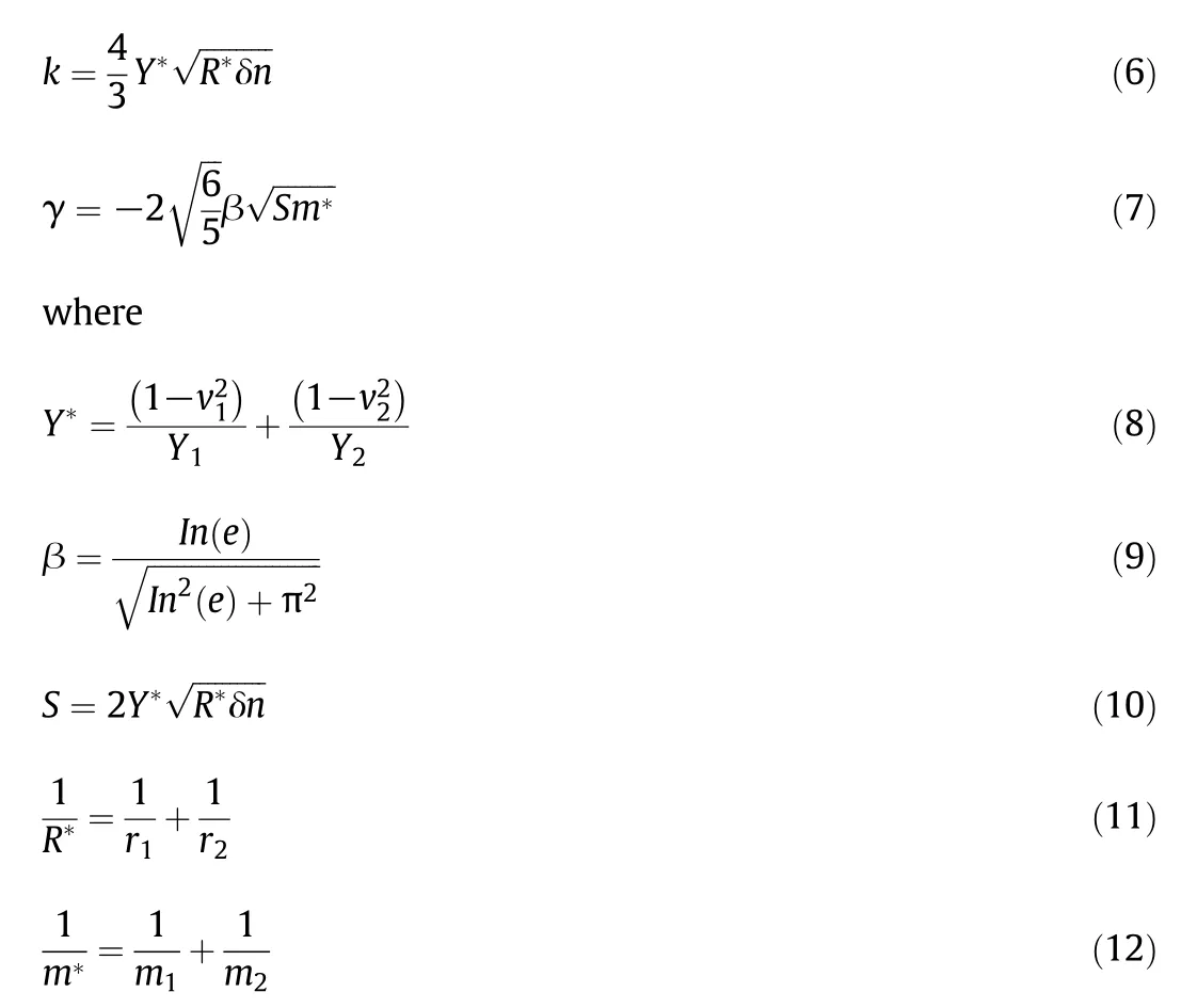
whereYis the Young's modulus,β is the momentum exchange coefficient,vis the Poisson ratio,andeis the coefficient of restitution,Riis the radius of particlei,andR*is the harmonic average radius of the particles.From equation(5),it can be seen that the rotational motion of particles has been ignored in this study.

In solid-liquid system,various forces may cause the formation of agglomerates,such as van der Waals force(vdw force)[25],liquid bridge force[26]and solid bridge force[27].Though the mechanism involved in this process is very complex,the primary effect is thought to be that of cohesion,that is,the attractive interactions between the particles.In this regard,a simple and representative form of the cohesive forces can be selected to characterize the cohesion between the particles(This point will be addressed further in Section IV and the Appendix).Here,the focus is on the relationship between the strength of the cohesion forces and the growth and breakage of agglomerates,whereas the detailed form of the forces has not been taken into account.In this work,the vdw force,which has been studied most,is taking as the representative cohesive force.It is only used as a model force rather than a physical reality.The vdw force model of Hamaker was used here to describe the cohesion between two particles with smooth surfaces,which is expressed as follows[28,29]:

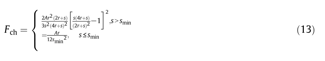
whereAis the Hamaker coefficient,a constant depending on the material properties.r=R1=R2is the radius of the two particles,sis the surface distance between the two particles,and the cohesive forceFchbecomes constant whens＜smin[28].The values ofAandsminaffect the intensity of agglomeration rather than the essential mechanism,therefore,they arefirst set as guessed values for polyethylene particles at 2.1×10-18J and 1.38×10-8m,respectively.The effects ofAare then investigated later on.

The sum of the pressure gradient force and the drag force is the fluid particle interaction force.By contrast to the pressure gradient force that is an output of DPM simulation itself,the drag force needs an input and in this study the well-known Wen-Yu's correlation is used[30]:

where the momentum exchange coefficient β is

where the drag coefficientCDis.

where the Reynolds numberRepdefined on the basis of the particle diameterdp= 2R,and the slip velocity between the particle and the surrounding fluid is

The simulation is carried out by coupling the in-house code of discrete element method for solid particles[31]with the open source code for the fluid flow,Open FOAM.The data exchange between these two programs is provided by shared memory with the help of mutex(mutual exclusion)semaphore in the Linux system.Therefore,DPM in this study is implemented in a highly parallel and efficient way.The finite-volume solver for the flow phase is executed on multi-core CPUs in the Mole-8.5 supercomputing system at IPE[32],whereas the highly parallel DEM solver for the solid phase is executed on its many-core GPUs to speed up the dynamic simulation,so the advantages of CPUGPU heterogeneous computing can be fully exploited.

Fig.1.Schematic diagram of the simulation domain in the experimental system.

3.Simulation Layout

In order to obtain a complete process of growth,stabilization and breakage of the agglomerates,ensuring a reasonable computational domain is important,hence a 25-millimeter-thick horizontal transport bed is simulated according to a lab-scale experimental facility at IPE and the operational experience from it[33].As shown in Fig.1,the simulated system includes an entrance(Domain 1),an expanding section(Domain 2),a stabilizing section(Domain 3-7),a narrowing section(Domain 8),and an exit finally.Its thickness is large enough to avoid its limitation to the agglomerates sizes,but still small enough to allow PIV(particle image velocimetry)measurements in the experiments for future comparison(which has not been carried out yet).The dimensions of the simulation domain are presented in Fig.1.When the simulation begins,mixed solid-liquid flow is transported into the reactor uniformly.Then agglomerates form,grow and break with the development of the flow.Finally,the particles and the fluid leave the reactor from the exit.The no-slip boundary condition for the fluid phase and the pressure-outlet boundary condition are used in the simulation.Nine GPU boards are used in the simulation,and every board corresponds to a computational domain as shown in Fig.1.It takes 3 to 7 days for each case,running at about 5×106particle-updates/sec in total.Table 1 shows more detailed parameters.

Table 1 Summary of the parameters used in the DPM simulations

4.The Flow Phenomena

The simulations are started from an empty reactor,therefore,it takes some times to reach a statistically steady state.We found that the flow and the agglomerates have reached a statistically steady state beforet=6 s.So in the following study all the results are based on the averaged value fromt=6 s tot=11 s.Fig.2 shows the position distribution of the particles marked with their velocities in the reactor att=11 s.It is evident that a substantial number of particles are not isolated,but aggregated into agglomerates with different sizes.To verify that this phenomenon is not specific to the vdw force used in this study,that is,this highly simplified model of the complex cohesive interactions between the particles is still representative,we also used the more realistic Simplified Johnson-Kendall-Roberts(SJKR)cohesion model to describe the cohesive force and simulated the same case.As described in the Appendix in detail,these two models gave qualitatively the phenomenon as long as comparable magnitudes of the cohesive forces were reached.The following discussions are,therefore,focused on the results from the vdw model.

The size and shape of the agglomerates change spatiotemporally,meanwhile particles may enter or leave agglomerates at any moment,as shown in Fig.3.The growth and breakage of the agglomerates must be controlled by the distribution of the forces.It is shown in Eq.(4)that the gravitational forceFg,the pressure gradient forceFp,the cohesive forceFch,the drag forceFdand the collision forceFclare considered to describe the behavior of particles.In the simulation,it was found that the order of the magnitude ofFgandFpare between 10-8N and 10-7N,and the order of the magnitude ofFch,FdandFclare between 10-5N and 10-4N.FgandFpare several orders of magnitude smaller than other forces,so it is believed thatFch,FdandFclare the major determinants of the growth and the breakage of agglomerates.For example,Fig.3(a)shows that a single particle collides with an agglomerate gently and then enters the agglomerate due to the cohesive force.Fig.3(b)shows that a particle leaves an agglomerate resulting from a strong collision by a high speed particle.Fig.3(c)shows that a particle leaves an agglomerate resulting from the traction of drag force.

5.Identification of Agglomerates

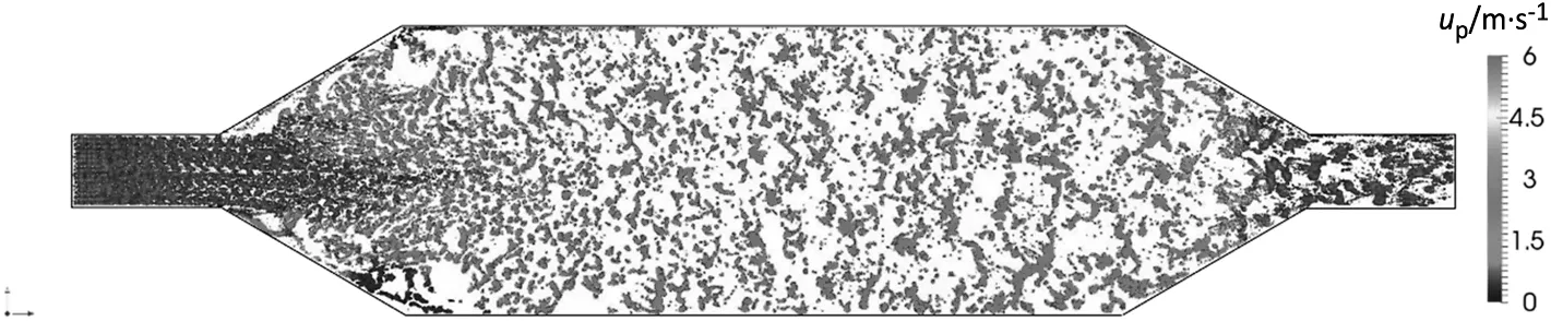
Fig.2.The position distribution of particles in the reactor.

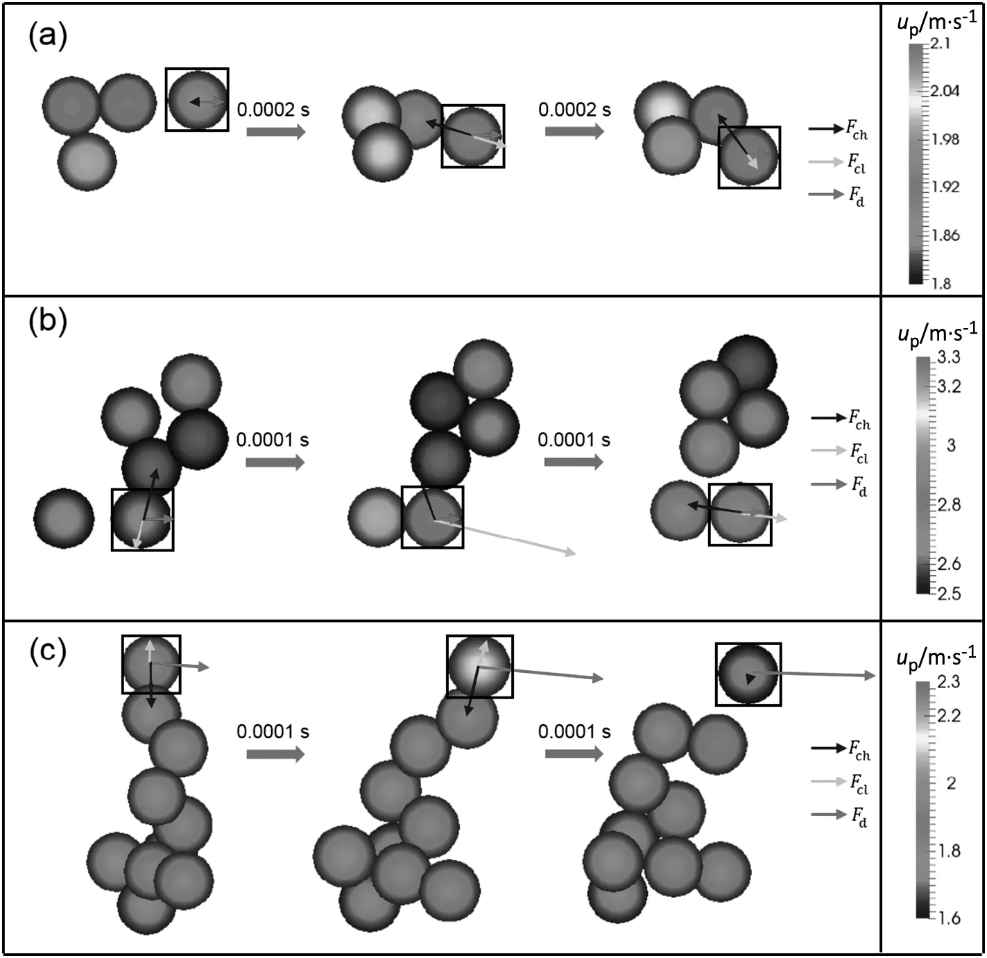
Fig.3.(a)Growth of an agglomerate after a weak collision resulting from cohesive forces,(b)breakage of an agglomerate resulting from strong collision,(c)breakage of an agglomerate resulting from the difference in the drag force.

Fig.4.The probability distribution of particles' contact time tr.

As has been indicated in the introduction,the dynamic evolution of agglomerates has a paramount effect on the hydrodynamics of the studied fluid-solid system,therefore,it is necessary to quantify the dynamic evolution of or the growth and breakage of agglomerates.In order to quantify the agglomerates,they should be identified first,therefore,in this section we provide a way to identify agglomerates.It is widely accepted that two cohesive particles form coordination when their surface distance is smaller than a certain value named as critical coordination distanced.There is however a controversy about the value ofd,but most scholars believe thatd=0 is a reasonable criterion[34,35].Apart from the distanced,the stability of coordination should be considered.For example,Liu proposed a method limiting the relative velocity of two particles[35].In DEM the duration of a contact can be measured and it is a more reasonable indicator of the stability of coordination.Since 5 s is much longer than the particles' residence time in an agglomerate,durations of all particle contacts in the reactor are counted from 6 s to 11 s,and its probability distribution is shown in Fig.4.There are two peaks on the distribution curve of the particle contact time,the first peak oftr=1.5×10-5s represents the short-time contacts(collisions)and the second peak oftr=2.5×10-4s represents the longtime contacts(agglomerates).The curve is at a low point whentris between 4×10-5s and 6×10-5s.Therefore,critical coordination timetc=5×10-5s is selected to remove the instantaneous collisions between particles.In summary,the agglomerate is determined bytc=5×10-5s andd=0 m for the simulation cases in this study.Although the value oftcis highly case-dependent,this method for determiningtcmay be of general applicability.

Fig.5.Spatial distribution of time-averaged particles number N p in an agglomerate.

6.Quantifying the Growth and Breakage of the Agglomerates

After identifying agglomerates,we could quantify the growth and breakup of agglomerates with known position of each particle at each time step.Fig.5 shows the spatial distribution of time-averaged particles numberNpin an agglomerate.At the entrance section fromx=0 mm to 100 mm,Npis close to 1,which indicates that almost no agglomerate forms due to the set homogeneous inlet boundary condition.When the flow reaches the expanding section fromx=100 mm to 330 mm,particles gather together to form small agglomerates with rapid growth rate.Then in the section fromx=330 mm to 480 mm,the growth of the agglomerates slows down and in the section fromx=480 mm to 730 mmNptends to stabilize at 35-40 roughly.Finally,at the exit fromx=730 mm tox=960 mm,the agglomerates break into small pieces due to the narrowing near the exit.In addition,in vertical direction of the flow,the size of the agglomerates is larger at the wall area than that at the center.The agglomerate size is controlled by a complex mechanism of agglomerate growth and breakage.The cohesive force is the primary driving force for agglomerate growth,enabling the agglomerates to attract other particles and stick with others.

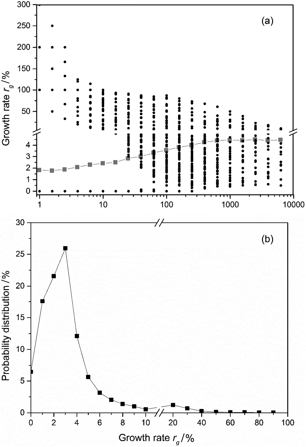
Fig.6.(a)The distribution of growth rate r g of agglomerates with different sizes,where the red squares represent mean values,(b)the distribution of growth rate r g of agglomerates including about 100 particles.

Fig.7.The distribution of the coordination number N C of the agglomerates with different sizes.

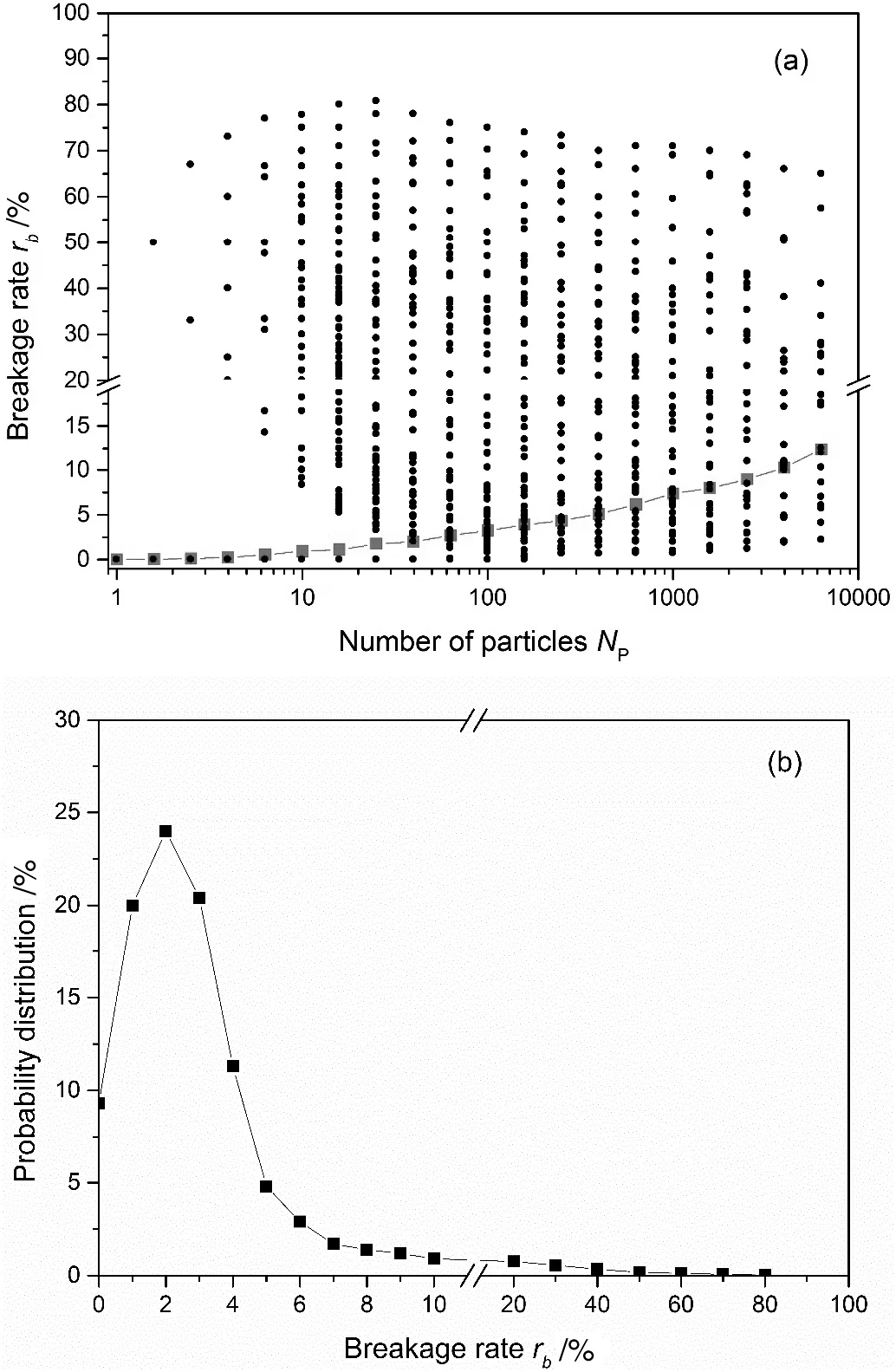
Fig.8.(a)The distribution of breakage rate r b of agglomerates with different sizes,(b)the distribution of breakage rate r b of agglomerates including about 100 particles.

The growth of an agglomerate is defined as that a single particle or a small agglomerate enter a large agglomerate,then the entering particles form coordination with particles of the original agglomerate.The original agglomerate refers to the agglomerate including most original particles after certain duration.The ability of an agglomerate to attract other particles can be quantified by its growth raterg.For an agglomerate,its growth ratergat timetis defined as the ratio of the numbers of the particles entering the agglomerate in the nextti=5×10-5s to the original particles number of the agglomerate at timet.Heretcshould be long enough to decrease the fluctuation of data and much shorter than the average residence time of the particles in the agglomerates.It is worth noting that the critical coordination timetcand the timetifor investigating the growth rate are not correlated,although their values are both 5×10-5s in this study.The relationship between the size and the growth rate of agglomerates is shown in Fig.6(a).The solid line is the averagedrgof agglomerates with different sizes.It can be seen that the larger the agglomerates,the larger its growth rate and ability to stick other particles,but once a certain critical value was reached,it levels off.The discrete points are the distribution ofrg. It can be seen that even for agglomerates of the same size,their growth rates are variable in a quite wide range resulting from the difference between their structures and environment.For example,Fig.6(b)shows the distribution of the growth ratergof the agglomerates including about 100 particles.The number of small agglomerates that was absorbed into the agglomerate is far larger than the number of large agglomerates.Furthermore,it can also be seen that the peak is at a growth rate of 3%,and in fact three single particles,a single particle and an agglomerate including two particles,or an agglomerate including three particles are all observed forms of the particles absorbed into the larger agglomerates.

Besides the size of the agglomerates,the structure and stability of the agglomerates have a significant effect on the growth and breakage of the agglomerates.Yang[36]believed that,there is bond energy between coordination particles in an agglomerate,which is destroyed during the breakage of the agglomerates.The total bond energy of a particle is related to its coordination numberNC, which is defined as the number of particles forming coordination with this particle.Therefore,the strength of an agglomerate is represented by its average coordination number of its member particles.The larger theNC, the larger the strength.Fig.7 shows the distribution ofNCof the agglomerates with differentsizes.The solid line is the averaged value ofNCof agglomerates with certain size.FromNp=2 toNp=600,NCand the strength of agglomerates increase together.WhenNpis larger than 600,NCand the strength of the agglomerates become approximately stable.The discrete points are the distribution ofNC.Even the agglomerates with same size,theirNCvalues may differ due to the different shapes,the one with largerNCis more compact and spherical.In addition,it is found that agglomerates with smallerNCoften emerge at the wall area with strong shearing caused by the presence of the no-slip wall.

Similar to the growth,the breakage of an agglomerate is defined as that a single particle or some particles leave a large agglomerate and the coordination no longer remains.For an agglomerate,its breakage raterbat timetis defined as the ratio of the numbers of the particles leaving the agglomerate in the nexttito the original particles number of the agglomerate at timet.

The relationship between the size and the breakage rate of the agglomerates is shown in Fig.8.It can be seen that the average breakage raterbincreases with the size of agglomeratesNP. Even for agglomerates of the same size,their breakage rates are variable in a quite wide range because of the difference of their structures and the surrounding fluid flow field.The breakage rate fluctuates between 0 and 80%,representing that no particle leaves the agglomerate and the agglomerate break thoroughly into many pieces,respectively.Furthermore,based on the results in Figs.6 and 8,the growth rate and breakage rate of most agglomerates are smaller than 20%,which indicates that the growth and breakage of most agglomerates are gradual process.

Fig.9 shows the average growth and breakage rates of the agglomerates as functions of the agglomerate size,and the probability distribution of the particle number in an agglomerate.The upper part of Fig.9(a)shows that whenNPis approximately 150,the average growth rate and breakage rate of the agglomerates are equal,and the probability distribution of the particle number in an agglomerate approximately peaks at this value also,as shown in the lower part of Fig.9(a).The conformance between the upper part and lower part of Fig.9(a)indicates statistically that the stable section of the reactor is long enough to ensure the dynamic balance of a large number of agglomerates.Fig.9,where simulations using various Hamaker coefficients and inlet velocities are conducted,summarizes all simulation results.It can be seen that when an agglomerate is smaller than the size at the cross point of the lines of the average growth rate and breakage rate,the growth rate is larger than the breakage rate,therefore,the size of the agglomerates more probably becomes larger.For an agglomerate larger than the size at the cross point,the average breakage rate is larger,thus the size of the agglomerate will more probably decrease.The dynamic equilibrium of agglomerate growth and breakage results in the peaked possibility in the bottom part of each picture in Fig.9.It can be concluded that at the cross point of the lines of growth rate and breakage rate,the number of particles entering and leaving an agglomerate are equal on average,so the growth and breakage of agglomerates achieve an dynamic equilibrium.This equilibrium exists widely in the stable section of the reactor and marks the most probable size of agglomerates.

Note that a nice framework for simulating an industrial system with dynamic agglomeration and breakage is the coupling of the two-fluid model and the population balance model[37].The results of the particle-level simulations reported in the present study can offer a significant insight into the growth and breakage of the particle agglomerates,which can be very helpful to the establishment of reasonable kernels for the population balance models describing these processes.These kernels are critical for the accuracy of this framework.

7.Conclusions

The discrete particle method is used to simulate a cohesive fluid particle flow and to quantify the growth and breakage of agglomerates.It was found that the growth and breakage of most agglomerates are step-by-step processes,while a few are abrupt changes.In addition,the most probable size of the agglomerates is determined by the balance of the growth and breakage of agglomerates,the cross point of growth and breakage rates as functions the particle number in an agglomerate marks the most stable agglomerate size.However,the underlying microscale mechanisms for the growth and breakage of agglomerates in cohesive fluid-particle systems are still unclear and need to be studied further,which should be related to the combination of the forces considered in DPM simulations and will be the topics of future study.Furthermore,the drag on the agglomerates may notbe accurately described by the correlations currently used,as has been demonstrated in heterogeneous gas-solid systems.How to develop more accurate correlations and whether they will amend the conclusions so far are also subject to future investigations.On the other hand,the present study is for an experimental system with only a section of the loop reactor in industrial processes,full loop simulation and analysis are highly desirable for practical application of the findings from this study.

Nomenclature

AHamaker coefficient,J

CDdrag coefficient

dcritical coordination distance,m

dpparticle diameter,m

ecoefficient of restitution

Fchcohesive force,N

Fclcollision force,N

Fddrag force,N

ggravity acceleration,m·s-2

knspring constant,N·m-1

mpparticle mass,kg

Nccoordination number

Npparticles' number in an agglomerate

plpressure,Pa

rparticle radius,m

rbbreakage rate of agglomerates,%

RepReynolds number

rggrowth rate of agglomerates,%

ssurface distance between two particles,m

smincut-off distance of the cohesion force,m

ttime,s

tccritical coordination time,s

tithe time for investigating the growth and breakage rate,s

trcontact time of particles,s

ulreal liquid phase velocity,m·s-1

upreal particle velocity,m·s-1

usslip velocity,m·s-1

vPoisson ratio

YYoung's modulus,Pa

βmomentum exchange coefficient,kg·m-3·s-1

εlVoidage

μlviscosity coefficient,Pa∙s

ρlliquid density,kg·m-3

τlliquid-phase stress tensor,kg∙m·s-2

Fig.10.The distribution of the particles in the reactor from the simulation using the SJKR cohesion model at t=11s.

Appendix

To verify that the choice of vdw force is representative,and this approximation does not change the nature of results,in this appendix we also choose Simplified Johnson-Kendall-Roberts(SJKR)cohesion model[38]to simply repeat the simulations in the main body of this work and compare their results.The cohesive force in the SJKR model is expressed as follows,F=k∙a,whereais the contact area of the particles,andkis the surface energy density.Again,ais calculated asa=2π∙s∙(2R*),wheresandR*are same to those in the Hamaker model.In the following simulation,we set surface energy density to 5000J∙m-3,and other parameters for the simulation layout are all the same to those for the Hamaker model.With these parameters,the mean magnitudes of the cohesion forces in both Hamaker and SJKR models are at the same order of 10-7N,while their cohesion energies are both at the same order of 10-15J.As shown in Fig.10 and compared to Fig.2,we con firm that,with a similar magnitude of the cohesion force,similar phenomenon of particle distribution and agglomeration can be obtained,at least for the steady states,so the simulation results in the main body of this work can be representative.

[1]J.R.V.Ommen,M.O.Coppens,C.M.V.D.Bleek,J.C.Schouten,Early warning of agglomeration in fluidized beds by attractor comparison,AIChE J.46(11)(2000)2183-2197.

[2]J.H.Li,M.Kwauk,Exploring complex systems in chemical engineering—The multiscale methodology,Chem.Eng.Sci.58(3-6)(2003)521-535.

[3]M.Horio,R.Clift,A note on terminology:‘clusters’and‘agglomerates’,Powder Technol.70(3)(1992)196.

[4]Y.Xiong,S.E.Pratsinis,Formation of agglomerate particles by coagulation and sintering—Part I.A two-dimensional solution of the population balance equation,J.Aerosol Sci.24(3)(1993)283-300.

[5]S.Heinrich,J.Blumschein,M.Henneberg,M.Ihlow,M.Peglow,L.Mörl,Study of dynamic multi-dimensional temperature and concentration distributions in liquidsprayed fluidized beds,Chem.Eng.Sci.58(23-24)(2003)5135-5160.

[6]F.Parveen,C.Briens,F.Berruti,J.Mcmillan,Effect of particle size,liquid content and location on the stability of agglomerates in a fluidized bed,Powder Technol.237(3)(2013)376-385.

[7]D.I.W.Pietsch,Agglomeration Processes:Phenomena,Technologies,Equipment,Wiley,2008.

[8]Z.Mansourpour,N.Mostoufi,R.Sotudeh-Gharebagh,Investigating agglomeration phenomena in an air-polyethylene fluidized bed using DEM-CFD approach,Chem.Eng.Res.Des.92(1)(2014)102-118.

[9]S.V.Manyele,J.H.Pärssinen,J.X.Zhu,Characterizing particle aggregates in a highdensity and high-flux CFB riser,Chem.Eng.J.88(1-3)(2002)151-161.

[10]R.Cocco,F.Shaffer,R.Hays,S.B.R.Karri,T.Knowlton,Particle clusters in and above fluidized beds,Powder Technol.203(1)(2010)3-11.

[11]M.Bartels,J.Nijenhuis,F.Kapteijn,J.R.V.Ommen,Detection of agglomeration and gradual particle size changes in circulating fluidized beds,Powder Technol.202(1)(2010)24-38.

[12]Y.J.Cao,Z.J.Shi,B.Z.Yang,C.G.Duan,J.D.Wang,Y.R.Yang,Detection of agglomeration in gas-phase polymerization fluidized-bed by using sound wave technique,Petrochem.Technol.35(8)(2006)766-769.

[13]T.Zhou,The calculation model of agglomerate sizes in fluidized beds of cohesive particles,Chem.React.Eng.Technol.15(1)(1999)44-51.

[14]S.Matsuda,H.Hatano,M.Tomoya,A.Tsutsumi,Modeling for size reduction of agglomerates in nanoparticle fluidization,AICHE J.50(11)(2004)2763-2771.

[15]S.Morooka,K.Kusakabe,A.Kobata,Y.Kato,Fluidization state of ultra fine powders,J.Chem.Eng.Jpn.21(1)(1988)41-46.

[16]K.Kuwagi,M.Horio,A numerical study on agglomerate formation in a fluidized bed of fine cohesive particles,Chem.Eng.Sci.57(22-23)(2002)4737-4744.

[17]T.Mikami,H.Kamiya,M.Horio,Numerical simulation of cohesive powder behavior in a fluidized bed,Chem.Eng.Sci.53(10)(1998)1927-1940.

[18]Y.Tatemoto,Y.Mawatari,K.Noda,Numericalsimulation of cohesive particle motion in vibrated fluidized bed,Chem.Eng.Sci.59(2)(2004)437-447.

[19]P.B.Tran,R.J.Miller,Onset of cohesive behavior in gas fluidized beds:A numerical study using DEM simulation,Chem.Eng.Sci.56(14)(2001)4433-4438.

[20]L.Q.Lu,J.Xu,W.Ge,Y.P.Yue,X.H.Liu,J.H.Li,EMMS-based discrete particle method(EMMS-DPM)for simulation of gas-solid flows,Chem.Eng.Sci.120(2014)67-87.

[21]Y.Tsuji,T.Kawaguchi,T.Tanaka,Discrete particle simulation of two-dimensional fluidized bed,Powder Technol.77(1)(1993)79-87.

[22]B.P.B.Hoomans,J.A.M.Kuipers,W.J.Briels,W.P.M.V.Swaaij,Discrete particle simulation of bubble and slug formation in a two-dimensional gas-fluidised bed:A hardsphere approach,Chem.Eng.Sci.51(1)(1996)99-118.

[23]B.H.Xu,A.B.Yu,Numerical simulation of the gas-solid flow in a fluidized bed by combining discrete particle method with computational fluid dynamics,Chem.Eng.Sci.52(16)(1997)2785-2809.

[24]P.A.Cundall,O.D.L.Strack,A discrete numerical mode for granular assemblies,Géotechnique29(1)(1979)47-65.

[25]P.A.Hartley,G.D.Par fitt,L.B.Pollack,The role of the van der Waals force in the agglomeration of powders containing submicron particles,Powder Technol.42(1)(1985)35-46.

[26]L.J.Mclaughlin,M.J.Rhodes,Prediction of fluidized bed behaviour in the presence of liquid bridges,Powder Technol.114(1)(2001)213-223.

[27]J.P.K.Seville,H.Silomon-Pflug,P.C.Knight,Modelling of sintering in high temperature gas fluidisation,Powder Technol.97(2)(1998)160-169.

[28]J.E.Galvin,S.Benyahia,The effect of cohesive forces on the fluidization of aeratable powders,AICHE J.60(2)(2014)473-484.

[29]H.C.Hamaker,The London—van der Waals attraction between spherical particles,Physica4(10)(1937)1058-1072.

[30]C.Y.Wen,Y.H.Yu,Mechanics of fluidization,Chem.Eng.Prog.Symp.Ser.62(1966)100-111.

[31]J.Xu,H.B.Qi,X.J.Fang,L.Q.Lu,W.Ge,X.W.Wang,M.Xu,F.G.Chen,X.F.He,J.H.Li,Quasi-real-time simulation of rotating drum using discrete element method with parallel GPU computing,Particuology9(4)(2011)446-450.

[32]W.Ge,J.Xu,Q.G.Xiong,X.W.Wang,F.G.Chen,L.M.Wang,C.F.Hou,M.Xu,J.H.Li,Multi-scale Continuum-particle Simulation on CPU-GPU Hybrid Supercomputer,Springer,Berlin Heidelberg,2013.

[33]J.H.Chen,R.T.Zhou,N.Yang,High concentrated liquid-solid flow in 2D bed for PE fluff swelling research,Technical Report,Institute of Process Engineering,CAS,2015.

[34]R.Y.Yang,A.B.Yu,S.K.Choi,M.S.Coates,H.K.Chan,Agglomeration of fine particles subjected to centripetal compaction,Powder Technol.184(1)(2007)122-129.

[35]D.Y.Liu,B.G.M.Van Wachem,R.F.Mudde,X.P.Chen,J.R.Van Ommen,An adhesive CFD-DEM model for simulating nanoparticle agglomerate fluidization,AICHE J.62(7)(2016)2259-2270.

[36]Y.Yang,Experiments and Theory on Gas and Cohesive Particles Flow Behavior and Agglomeration in the Fluidized bed System,PhD Thesis,Illinois Institute of Technology.,1991

[37}R.Fan,D.L.Marchisio,R.O.Fox,Application of the direct quadrature method of moments to polydisperse gas-solid fluidized beds,Powder Technol.139(2004)7-20.

[38]K.L.Johnson,K.Kendall,A.D.Roberts,Surface energy and the contact of elastic solids,Pros.R.Soc.Lond.A.324(1971)301-313.