Effects of heterogeneity distribution on hillslope stability during rainfalls

Jing-sen Ci,E-chun Yn,Tin-chyi Jim Yeh*,Yun-yun Zh

aFaculty of Engineering，China University of Geosciences，Wuhan 430074，China

bDepartment of Hydrology and Water Resources，University of Arizona，Tucson，AZ 85721，USA

Received 28 September 2015；accepted 3 March 2016

Available online 22 June 2016



Effects of heterogeneity distribution on hillslope stability during rainfalls

Jing-sen Caia,E-chuan Yana,Tian-chyi Jim Yehb,*,Yuan-yuan Zhab

aFaculty of Engineering，China University of Geosciences，Wuhan 430074，China

bDepartment of Hydrology and Water Resources，University of Arizona，Tucson，AZ 85721，USA

Received 28 September 2015；accepted 3 March 2016

Available online 22 June 2016

Abstract

The objective of this study was to investigate the spatial relationship between the most likely distribution of saturated hydraulic conductivity(Ks)and the observed pressure head(P)distribution within a hillslope.The cross-correlation analysis method was used to investigate the effects of the variance of lnKs,spatial structure anisotropy of lnKs,and vertical infiltration flux(q)on P at some selected locations within the hillslope.The cross-correlation analysis shows that,in the unsaturated region with a uniform flux boundary,the dominant correlation between P and Ksis negative and mainly occurs around the observation location of P.A relatively high P value is located in a relatively low Kszone,while a relatively low P value is located in a relatively high Kszone.Generally speaking,P is positively correlated with q/Ksat the same location in the unsaturated region.In the saturated region,the spatial distribution of Kscan significantly affect the position and shape of the phreatic surface.We therefore conclude that heterogeneity can cause some parts of the hillslope to be sensitive to external hydraulic stimuli(e.g.,rainfall and reservoir level change),and other parts of the hillslope to be insensitive.This is crucial to explaining why slopes with similar geometries would show different responses to the same hydraulic stimuli,which is significant to hillslope stability analysis.

©2016 Hohai University.Production and hosting by Elsevier B.V.This is an open access article under the CC BY-NC-ND license(http:// creativecommons.org/licenses/by-nc-nd/4.0/).

Cross-correlation analysis；Heterogeneity；Hillslope stability；Saturated hydraulic conductivity；Stochastic conceptualization；Pore-water pressure

1.Introduction

Spatial variability of hydraulic properties of geologic media(e.g.,the presence of macropores,fractures,folds, fissures,layers,preferential flow paths,and clay lenses)is the rule rather than the exception.Even seemingly uniform field sites show a high degree of spatial variation in the saturated hydraulic conductivity value(Nielsen et al.,1973). Such variability controls hillslope soil strength distribution,groundwater flow,pore-water pressure distribution,and seepage force,and,in turn,plays a salient role in hillslope stability along with other factors such as spatial and temporal variability of precipitation.As such,this information allows determination of stress distribution within a hillslope,and appropriate actions can be taken to mitigate possible failure of the hillslope.While the importance of the spatial variability or heterogeneity is well known,it is practically impossible to describe these heterogeneities in detail.In order to overcome this difficulty,probabilistic methods,or methods based on random or stochastic field theory,have been employed in hydrogeology and geotechnical engineering(Yeh,1992；Gelhar,1993；Griffiths and Fenton,1993, 2004；Gui et al.,2000；Srivastava et al.,2010；Cho,2012；Zhu et al.,2013；Yeh et al.,2015).For example,the random finite element method(RFEM),proposed by Griffiths and Fenton(1993)and Fenton and Griffiths(1993),has been widely used to consider the spatial fluctuations of a parameterin hillslope stability analysis(Gui et al.,2000；Cho,2012, 2014；Zhu et al.,2013).

Generally,for a given hillslope,one may collect soil samples at some locations to determine spatial statistics of hydraulic parameters；these spatial statistics are then used to infer the spatial variability of hydraulic parameters across and throughout the hillslope.From the given spatial statistics of the parameters,one can generate many possible spatial distributions of the parameters of the hillslope.Of these distributions,some are favorable to slope stability,and some are not for given rainfall events.In practice,it is rather costly and difficult to characterize the hydraulic heterogeneity by taking soil samples；on the other hand,it is relatively inexpensive and typical to observe hydraulic responses/states,such as the pore-water pressure at hillslope toes or the position of phreatic surface at some locations.As a matter of fact,pore-water pressure distributions are one of the major stresses that control the hillslope stability.This simple reality thus compels us to ask,what can be inferred about the likely spatial distribution of saturated hydraulic conductivity within a hillslope from some observed hydraulic responses or pore-water pressures at some locations within the hillslope？

Zhu et al.(2013)carried out a probabilistic infiltration analysis considering a spatially varying permeability function within a two-dimensional(2D)hillslope.With one set of given statistical parameters,they showed the spatial distributions of saturated hydraulic conductivity that can lead to the highest and lowest groundwater tables in the hillslope.However,they did not focus on the effects of the spatial distribution of saturated hydraulic conductivity in various hydraulic scenarios,nor did they investigate the relationship between the likely distribution of saturated hydraulic conductivity and observed pore-water pressures at some given locations within a hillslope.

Cross-correlation analysis can serve as a quantitative tool for answering the question posed above.Cross-correlation analysis has been widely used by hydrogeologists over the past decade.For example,Yeh et al.(2014)used a simple example to elucidate the cross-correlation relationship between the observed heads in a saturated aquifer and the hydraulic conductivity in a one-dimensional aquifer.Mao et al. (2011)conducted cross-correlation analysis to investigate how the spatial variability of hydraulic parameters,such as the saturated hydraulic conductivity,specific storage,and saturated moisture content,at different locations in unconfined aquifers affect the head at a given location in the unsaturated and saturated regions.Wu et al.(2005)and Sun et al.(2013) used cross-correlation analysis to study the spatial and temporal evolution of cross-correlations between soil properties (transmissivity and storage coefficients)and the head responses at an observation well during a pumping test,in both homogeneous and heterogeneous aquifers.

At present,few have attempted to study the ways in which the saturated hydraulic conductivity at different locations within a hillslope influences the pore-water pressure at some crucial locations within the hillslope.More importantly,few studies have quantified the relationship between the most likely distribution of saturated hydraulic conductivity and the observed pressure head distribution within a hillslope subject to rainfalls or other external events.This relationship may allow us to better control the pore-water pressure distribution within a hillslope.

The objectives of this study were therefore(1)to examine how the pressure head at a crucial location(e.g.,the slope toe) is affected by the saturated hydraulic conductivity at different locations within a hypothetical hillslope；(2)to investigate the relationship between the most likely distribution of saturated hydraulic conductivity and the observed pressure head distribution within a hillslope；and(3)to elucidate the likely distribution of saturated hydraulic conductivity and the flow field distribution within a heterogeneous hillslope subject to some given hydraulic events,which are critical to the study of hillslope stability.

2.Methodology

2.1.Governing equation

While transient flow is more realistic,for the sake of simplicity and a first cut analysis,in this paper we focus on steady-state flow in a heterogeneous hillslope,which is pertinent to long-term status analyses.Here,we assume that the flow in a heterogeneous 2D vertical hillslope cross-section can be described by the following equation:

and is subject to the following boundary conditions:

where P is the pressure head；z is the elevation head；K(P) is the hydraulic conductivity-pressure constitutive function；PDis the prescribed pressure head at the Dirichlet boundary ΓD；qNis the specific flux at the Neumann boundary ΓN；and nxand nzare the components of the unit vector n in the x and z directions,respectively,and n is normal to the boundary ΓN.

2.2.Moisture retention and hydraulic conductivity functions

In order to simulate flow in a hillslope using Eqs.(1)and (2),the moisture retention and hydraulic conductivity curves developed by van Genuchten(1980)and Mualem(1976), respectively,also known as the MVG model,are adopted here, and can be expressed as

where α,n,and m are soil parameters,and m=1-1/n；θ(P)is the volumetric water content；θsand θrdenote the saturated and residual moisture contents,respectively；and Ksis the saturated hydraulic conductivity.

2.3.Random field theory

2.3.1.Stochastic conceptualization of heterogeneity

Hydraulic properties generally exhibit a high degree of spatial variability at various scales(Nielsen et al.,1973；Bouwer,1978；Yeh,1992；Cho,2012).As a result,accurate analysis of flow or stability analysis of a hillslope would require detailed characterization of the hillslope.Nevertheless, it is impossible to sample and map hydraulic properties at every location within a hillslope.We therefore have to estimate or guess their values at a location if there is no measurementoftheproperty (forexample,Ks)orif its measurement involves error.Our guess or estimate inevitably causes us to unknowingly conceptualize Ksat the location as a random variable,characterized by a probability distribution. While the probabilistic conceptualization of Ksis rational,the fact is that Ksat a given location,even if it has been determined exactly,can always be treated as a random variable. This is tantamount to stating that the value of Ksdetermined at that location represents just one of the many possible values of Ksof geologic materials that may have been deposited at this location when the environment comes into existence.Therefore,a hydraulic property of a geologic formation at a given location can always be considered a random variable regardless of whether the property is known or whether it involves measurement error.As a consequence,the hydraulic conductivity field within a hillslope can be considered a collection of random variables.This collection of an infinite number of random variables is then called a stochastic process,or random field.A more detailed introduction of stochastic conceptualization of heterogeneity is provided in Yeh et al.(2015).

Following the procedure of Yeh et al.(2015),in order to describe Ksheterogeneity within a hillslope as a random field, weimplicitlyassumethattherandomfieldhasajointlognormal distribution,which is characterized by a mean（μKs）,a varianceand a correlation structure described by a covariance function with some correlation scales(λ).Furthermore,we let the natural logarithm of saturated hydraulic conductivity,lnKs, be F；it has a meanand perturbation,f,whose variance is denoted by.Furthermore,F is assumed to have a statistically isotropic or anisotropic covariance,which is described by an exponential covariance function:

where R(A,A′)is the autocovariance function of F at points A and A′,located at(x,z)and(x′,z′),respectively；and λxand λzare the correlation scales in the x and z directions,respectively.

The autocovariance function of F is a statistical measure of the spatial structure(or spatial pattern)of F heterogeneity. That is,it describes how the value of F at one location is related to the F values at other locations.Physically,the correlation scales of F then represent the average dimensions (e.g.,length and thickness)of heterogeneity(e.g.,layers or stratifications).

Although other parameters such as α,n,θs,and θrof the MVG model(Eqs.(3)and(4))do exhibit spatial variability (Yeh et al.,2015),in this analysis,we assumed that their spatial variability had insignificant effects on hillslope stability issues and they were assumed to be constant throughout the hillslope(Gui et al.,2000；Mao et al.,2011；Cho,2012,2014；Zhu et al.,2013).

2.3.2.Random field generation using fast Fourier transformation

In order to generate a random field,a fast Fourier transform code modified from Gutjahr(1989)is used,which is computationally efficient(Zhu et al.,2013)and can produce a reasonable and discretized random field with a defined mean and variance,as well as correlation scales.The random field is represented in the form of discretization,in which the hydraulic conductivity in the random field is generated at each element for finite element analysis.Each realization of the random field is first generated in a rectangular domain,with the same width and height as the hillslope,and then the region outside the boundary of the hillslope is truncated.Thus,a realization with the geometry of the hillslope is generated, following the approach of Zhu et al.(2013).

2.4.Cross-correlation analysis

Cross-correlation analysis(Zhang and Yeh,1997；Li and Yeh,1998；Hughson and Yeh,2000；Mao et al.,2011；Sun et al.,2013)has been carried out to investigate how the pressure head at a given location is affected by Ksat different locations within a hillslope,based on a Taylor series expansion of the flow model(Eq.(1)).Since natural logarithms of saturated hydraulic conductivity,lnKs,at different locations within the hillslope are treated as a random field with some spatial correlation,we express them as lnKs=F=+f, where f represents the spatial variability or uncertainty due tolack of measurements of Ksor lnKs.Likewise,the pressure head is represented by P=+p,whererepresents the mean pressure head within an equivalent homogeneous hillslope,evaluated usingand p denotes the perturbation of pressure head.Subsequently,the pressure head can be expanded in a Taylor series regarding:

To reduce the computational load,the sensitivity was calculated with a numerical adjoint state method(Sykes et al., 1985；Li and Yeh,1998,1999；Hughson and Yeh,2000)in this study.

Multiplying Eq.(7)with itself,and based on the following expectation:

where i,k=1,2,…,N,and j,l=1,2,…,M,we generate the following relation:

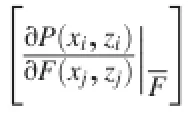
Similarly,multiplying Eq.(7)with f(xl,zl)and with the following expectation:

we obtain the cross-covariance between the pressure head P at the location(xi,zi)and lnKsat the location(xl,zl):

where［Rpf］represents the cross-covariance function matrix between the pressure head P and lnKs.

Rpfis normalized by the square root of the product ofandto obtain the corresponding crosscorrelation ρpf:

where［ρpf］is the cross-correlation function matrix between the pressure head P and lnKs.

Here we must point out that this cross-correlation analysis is based on the first-order approximation,which ignores the higher-order terms in the Taylor series.As a computationally efficient approach,this cross-correlation analysis has been widely used in inverse modeling as well as joint inversion of flow,solute transport,and geophysical surveys.

2.5.Procedure to select corresponding realization for given hydraulic scenario

There are an infinite number of realizations of Ksfields of a heterogeneous hillslope with the same prescribed statistical parameters.When a certain hydraulic scenario,for example, the pressure head at the hillslope toe reaching its maximum,is selected,few realizations may exist whose hydraulic responses satisfy this hydraulic scenario.To select these possible realizations,we take advantageofthepreceding crosscorrelation analysis.

According to Eq.(7),we know that the pressure head P at one location is influenced by Ksor lnKsat different locations within a hillslope.The cross-correlation ρpf＞0 means thatan increase in Ksor lnKsat the location(xj,zj)can lead to an increase in the pressure head P at the selected location(xi,zi) within the hillslope and vice versa(positively-correlated), while ρpf＜0 means that an increase in Ksor lnKsat the location(xj,zj)produces a decrease in the pressure head P at the selected location(xi,zi)and vice versa(negatively-correlated),and ρpf=0 means no connection between Ksor lnKsand the pressure head P.That is,the cross-correlation ρpfcould be considered normalized weights,which quantify the influences of Ksor lnKsat different locations on the pressure head P at some selected crucial locations within the hillslope.

Accordingly,a criterion Aeis set up to select the realization that best meets the requirement of a hydraulic scenario:

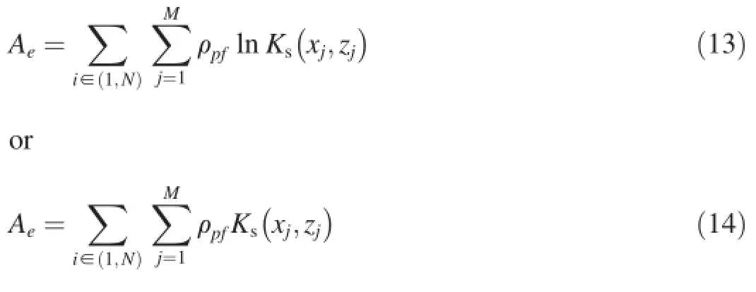
where e=1,2,…,L,which denotes the numbers of generated realizations of Ksfields of the hillslope.i∈(1,N)means that the selected crucial locations for the pressure heads could be a point group or just one point.For each realization of the Ksfield within the hillslope,Aecould be calculated with Eq.(13) or Eq.(14).The maximum of Aeindicates that the pressure head at the selected location reaches a maximum,and the minimum of Aeindicates that the pressure head at the selected location reaches a minimum.That is to say,Aecan be used as the criterion for selection of a realization, which satisfies the given hydraulic scenario,from an infinite number of realizations with the same prescribed statistical parameters.

In fact,there may exist other possible realizations that satisfy the given hydraulic scenario,and the selected realization may not be unique.Here we merely use this procedure to select some realizations for illustration purposes.That is,we want to demonstrate what the likely distributions of saturated hydraulic conductivity and flow field within a heterogeneous hillslope might look like for some given critical hydraulic scenarios,with different rainfall amounts and spatial statistics, which describe the heterogeneous nature of saturated hydraulic conductivity within the hillslope.

3.Setup of simulations

3.1.Model and parameters

In order to investigate the relation between the most likely distribution of saturated hydraulic conductivity and the observed pressure head distribution within a hillslope, several numerical experiments were conducted.All the experiments were based on a synthetic 2D vertical cross-section of a hypothetical hillslope.Fig.1 displays the geometry and boundary conditions of the hillslope.The boundaries AH and BC are the Dirichlet boundaries with constant heads,that is,（P+z）|AH=20m,and（P+z）|BC=10m.The boundary AB is impermeable,and the boundary GF is the Neumann boundary with a constant vertical flux q.The boundaries FE, ED,GH,and DC are defined as seepage faces.The boundaries FE and ED vary from the Neumann boundaries with constant q in the unsaturated state to boundaries with zero pressure head in the saturated state.The boundaries GH and DC vary from impermeable boundaries in the unsaturated state to boundaries with zero pressure head in the saturated state.The simulation domain(100 m×40 m)in the vertical plane is evenly discretized into 50×40 elements and 2091 nodes,and then the top right corner of the domain is truncated.Thus,the shape of the remaining part with 1610 elements and 1681 nodes becomes the geometry of the hillslope (Fig.1).

Stochastic representation of the heterogeneous hillslope (as discussed in the preceding section)was used to provide a quantitative but bulk description of the heterogeneity within the hillslope.μKswas set to 1.0 m/d.The values of soil hydraulic parameters,set to be uniform in this study,were as follows:α=0.4 m-1,m=0.5,n=2,θr=0.07,and θs=0.4. Table 1 lists the spatial statistics of Ksused in the numerical experiments.In this study,only Kswas treated as a random field,although other parameters also exhibited spatial variability.These statistical values were selected based on comprehensive surveys of literature on spatial variability of unsaturated hydraulic parameters,as summarized in Yeh et al. (2015).Based on published studies(Nielsen et al.,1973；Rawls et al.,1982；Carsel and Parrish,1988；U¨nlu¨et al., 1990；White and Sully,1992；Russo and Bouton,1992；Khaleel and Freeman,1995；Russo,1997；Gui et al.,2000；Srivastava et al.,2010；Santoso et al.,2011；Cho,2012；Zhu et al.,2013),a general range of 30%-100%of the coefficient of variation(CV=σKs/μKs)of Kswas suggested.Thus, the general range of variance of lnKscould be 0.1 to 0.7,and we also used a high variance of 1.5 for comparison.Correlation scales of 0.025-100 times the slope height were suggested for lnKs,which were 0.5-2000 m in Zhu et al.(2013). Actually,not only the slope height,but also the grid size and entire domain size needed to be considered to determine aproper correlation scale.Meanwhile,the anisotropy of lnKscould not be neglected.In this study,the correlation scale of lnKsin the vertical direction,λv,was determined to be 10 m, and the correlation scale of lnKsin the horizontal direction, λh,was changed from 10 to 100 m.The ratio between the vertical infiltration flux q and μKswas set to 0.01(mild rainfall intensity)based on Zhu et al.(2013),and we increased this value to 0.05 for comparison purposes.These small values are shown to be able to maintain a constant matric suction in the unsaturated region(Zhang et al.,2004), and make the constant infiltration flux boundary realistic.

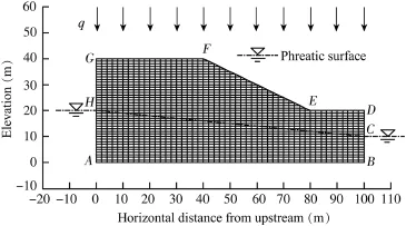
Fig.1.Hypothetical hillslope in numerical study.

Table 1Study cases.

In the analysis,the six cases listed in Table 1 were used in parametric studies on the effect of three factors,which were the variance,spatial structure anisotropy(λh/λv),and normalized vertical infiltration flux（q/μKs）.More specifically,cases 1 and 2 focused on the effects of the variation of；cases 1,3,and 4 focused on the effects of the variation of λh/λv；and cases 1,5,and 6 focused on the effects of the variation of q/μKs.

A finite element numerical model code for simulating variably saturated flow and transport in two dimensions (VSAFT2),presented by Yeh et al.(1993),with the corresponding software available at www.hwr.arizona.edu/yeh,was used to simulate flow fields for the hillslope scenario.This program solves Eq.(1)with nonlinear finite element approximation based on the Newton-Raphson method.The program also includes an iterative scheme,since it needs to arrive at the appropriate boundary condition along seepage faces(Rulon and Freeze,1985).

3.2.Flow field within a homogeneous hillslope

To present a basic understanding of the flow field within the hypothetical hillslope,we first simulated the steady flow in the hillslope,in which the Ksvalues of all elements were assumed to be the mean saturated hydraulic conductivity (i.e., μKs=1.0 m/d),other parameters were assumed to be uniform, and the vertical infiltration flux was q=0.01 m/d.Fig.2 shows the simulated flow field,including streamlines(or flow lines),contour lines of pressure head,and the phreatic surface.The flow field derived from the homogeneous mean parameter values represents the most likely flow field with given infiltration rates and boundary conditions.Although this most likely field can be quite different from the field based on heterogeneous parameters,it displays the general flow field within the hillslope.

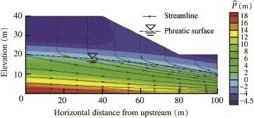
Fig.2.Mean pressure head evaluation for homogeneous hillslope when Ks=μKs=1.0 m/d.

4.Results and discussion

4.1.Cross-correlation analysis

First,we used cross-correlation analysis to investigate how the pressure head at a location is affected by Ksor lnKsat differentlocationswithinthehypotheticalhillslopeincase1.As shown in Fig.3(a),the spatial distribution of cross-correlation between lnKsat different locations and P with the observation location at the slope toe is used to represent the situation in the unsaturated region,while the spatial distribution of crosscorrelation with the observation location of P under the slope toe,belowthemeanpositionofthephreaticsurface,asshownin Fig.3(b),is representative of the situation in the saturated region.Fig.3indicatesthatthedistributionofcross-correlationfor the pressure head observation location in the unsaturated region is quite different from that for the pressure head observationlocation in the saturated region；however,the distributions of cross-correlation have similar characteristics in the unsaturated region and saturated region,respectively,regardless of the pressure head observation location.

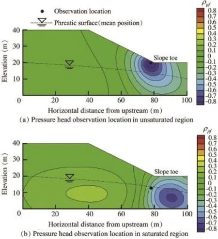
Fig.3.Spatial distributions of cross-correlation between lnKsand P in steady state for case 1.

As illustrated in Fig.3(a),in the unsaturated region,the pressure head is negatively correlated with lnKsin the region around the pressure head observation location at the slope toe, with a cross-correlation value reaching-0.8.As the distance from the pressure head observation location(e.g.,the slope toe) increases,the cross-correlation values tend to be less negative, showing a decreasing correlation,and finally become slightly positiveintheupstreamregion.Overall,thepressureheadatthe slope toe is dominated by negative cross-correlation with lnKs. These results also demonstrate that the pressure head at an observation location within the hillslope is not equally influencedbyheterogeneity everywherewithinthehillslope,andthe most influenced region is around the pressure head observation location at the slope toe,as shown in Fig.3(a).

As shown in Fig.3(b),in the saturated region,the pressure head at the observation location is positively correlated with lnKsin the upstream region and negatively correlated with lnKsin the downstream region.This pattern of correlation follows the direction of the streamline(see Fig.2 for the streamline).This result is consistent with the findings in Li and Yeh(1999)and Mao et al.(2011).Specifically,the pressure head is positively correlated with Ksin the up-gradient region and negatively correlated with Ksin the down-gradient region with respect to the pressure head observation location along the streamline toward the pumping well.Here,the drain outlet of the downstream slope is equivalent to a pumping well.Yeh et al.(2014)used a simple example to elucidate this relationship.

4.2.Effect of three factors on results of cross-correlation analysis

For cases 1 through 6 in Table 1,cross-correlation analysis was used to investigate the degree of influence of lnKsat different locations within the hillslope on the pressure head with the observation location at the slope toe in the steady state.The resultant spatial distributions of cross-correlation within the hillslope for the six cases are shown in Fig.4. Note that,λh/λv,and q/μKshave similar effects when the pressure head observation location is in the saturated region.

Comparison of case 1 and case 2 in Fig.4 indicates thathas no effect on the spatial distribution of cross-correlation between lnKsand P.This is due to the fact that the crosscorrelation value is obtained by normalizing the cross-covariance Rpfusing the square root of the product of and.

When we compare case 1,case 3,and case 4,we find that, with the increase of spatial structure anisotropy,λh/λv,the pattern of spatial distribution of cross-correlation becomes more stratified.When the observation location of pressure head is in the unsaturated region,the negatively correlated region increases with the value of λh/λv,and the crosscorrelation value between lnKsand P of the whole region within the hillslope becomes more negative.The positively correlated region,formerly existing in the upstream region,is gradually covered by the negatively correlated region with the increase of λh/λv.The reason for these phenomena is that,with the increasing spatial structure anisotropy of Ks,the autocorrelation between Ksat any two locations increases,leading to the increase of the negatively correlated region.

Comparisons of case 1,case 5,and case 6 demonstrate that an increase in the vertical infiltration flux q changes the spatial distribution of cross-correlation between lnKsand P.More specifically,the negatively correlated region increases with the value of q,and the most negative value of cross-correlation becomes less negative.This result can be attributed to the fact that the flow fields are different for different vertical infiltration fluxes.However,this change is not very dramatic.

4.3.Spatial distribution pattern of saturated hydraulic conductivity with respect to pressure head within a heterogeneous hillslope

Based on the spatial distributions of cross-correlation in Figs.3(a)and4,wecanfurtherconcludethat,intheunsaturated region,subject to a constant flux(or Neumann)boundary,the location with a relatively high P is in a relatively low Kszone, while the location with a relatively low P is in a relatively high Kszone.Thiscanbeattributedtothefactthat,intheunsaturated region,the dominant correlation between P and Ksis negative and mainly occurs around the pressure head observation location.The matric suction(i.e.,the absolute value of negative pore-waterpressure)inarelativelylowKszoneislow,andthere may evenexisthighpositivepressures.Therefore,therelatively low Kszones inthe unsaturatedregionclose tothe slopesurface arethemorelikelydeformationandfailurezones,whichrequire special attention and prevention.

On the other hand,based on Fig.3(b),we can determine that,in the saturated region subject to a constant pressure head (or Dirichlet)boundary,if a location has a relatively high P or is under a relatively high phreatic surface,the upstream region is a relatively high Kszone while the downstream region is a relatively low Kszone.Meanwhile,if the P value or the phreatic surface is relatively low at a location,a relatively high Kszone exists downstream,while a relatively low Kszone exists upstream.

Note that this spatial distribution pattern of Ksis valid only for the boundary conditions considered here.For example,if we assign a constant head(or Dirichlet)boundary along GF, FE,or ED(Fig.1)in the unsaturated region(e.g.,pond and surface water),then the pattern in the unsaturated region will be similar to that in the saturated region.As a result,the pattern depends on the boundary condition.

4.4.Examples of realizations for given hydraulic scenarios

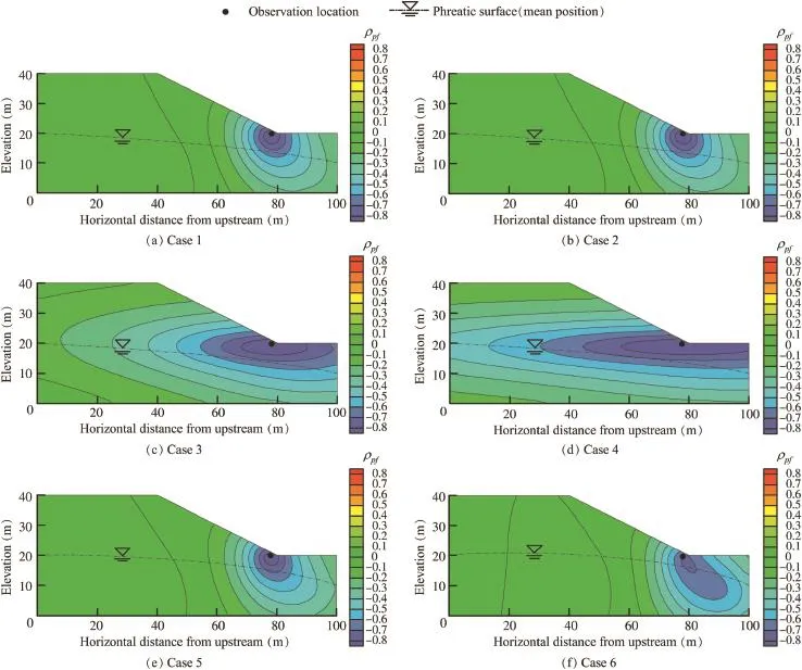
Fig.4.Spatial distributions of cross-correlation between lnKsat different locations and P at slope toe in steady state for different cases.

Using the procedure to select realizations for given hydraulic scenarios(Eq.(13)or(14)),realizations of Ksfields and the corresponding flow fields for the six cases that satisfy the hydraulic scenarios,in which the pressure head at the slope toe reaches a maximum or minimum,were obtained.Ten thousand realizations were generated for each case.We must emphasize that here the hydraulic scenario focused on just the slope toe,the only observation location within the hillslope.If the target changes or expands,the selected realizations will change.

4.4.1.Pressure head at slope toe reaching maximum

Fig.5 shows the selected Ksrandom fields and their corresponding flow fields,conditioned to the scenario in which the pressure head at the slope toe is maximum.As illustrated in Fig.5,the selected realizations for the six different cases all have high Ksvalues in the upstream region and low Ksvalues in the downstream region,and the slope toe is located in a relatively low Kszone.In the unsaturated region,a relatively low P value tends to exist in a relatively high Kszone.Such spatial distributions of Ksare consistent with the crosscorrelation pattern between Ksand P,and correspond to the maximum pressure head at the slope toe under the prescribed boundary conditions.

In addition,for case 1,shown in Fig.5(a),the Ksfield fluctuates spatially,each high/low Kszone is surrounded by other low/high Kszones,and there appears to be no preferential distribution direction.This is reasonable in realistic conditions when this slope soil profile is within regionally similar deposits without a specific depositional direction. Case 2 shows the spatial distribution of Kssimilar to that in case 1,but with a greater difference between the high Ksvalue and the low Ksvalue within the hillslope(i.e.,greater heterogeneity).The spatial distributions of Ksin cases 3 and 4 are horizontally stratified,representing a horizontally layered slope,although in case 3 there exist some small discontinuities(e.g.,high Kszone-like fractures and low Kszone-like barriers)in each layer.The spatial distributions of Ksin cases 5 and 6 are similar to that in case 1,since their crosscorrelation patterns are similar,as illustrated in the preceding section(Figs.4(a),(e),and(f)).

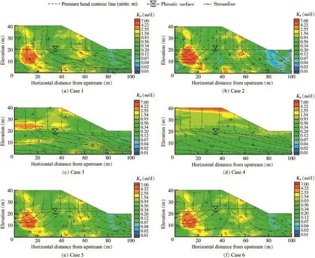
Fig.5.Spatial distributions of realized Ksfields and flow fields in steady state for different cases,subject to hydraulic scenario in which pressure head at slope toe reaches a maximum.

Comparing case 1 with case 2 in Fig.5,we find that a higherleads to a greater difference between the high Ksvalue and the low Ksvalue within the hillslope.This also results in a higher phreatic surface and a higher pressure head at the slope toe.

Comparisons of case 1,case 3,and case 4 in Fig.5 demonstrate that when the Ksrandom field of selected realizations becomes more stratified,the field tends to show smooth variation within the horizontal layers,and the Ksvalues tend to be low in most regions of the hillslope,especially in the saturated region below the phreatic surface.This leads to a lower phreatic surface and a lower pressure head at the slope toe.Moreover,the corresponding streamlines become straighter and smoother,making them similar to the streamlines in the homogeneous hillslope in Fig.2.These results suggest that an isotropic hillslope with relatively small correlation scales may produce a small number of patches of high positive pressure in the unsaturated region,which are localized and hard to detect,but may be critical for slope stability analysis.On the other hand,horizontally layered slopes are more likely to produce large-scale hydraulic features(e.g.,perched water table aquifers),which are easier to detect.

Comparisons of case 1,case 5,and case 6 in Fig.5 indicate that an increase in the vertical infiltration flux q produces a higher phreatic surface and a higher pressure head at the slope toe.

4.4.2.Pressure head at slope toe reaching minimum

Fig.6 shows heterogeneous Ksfields and their corresponding flow fields,subject to the condition that the pressure head at the slope toe must be at a minimum.Each realization for each case in Fig.6 has similar characteristics of spatial distribution of Ksto that in Fig.5.However,unlike the realizations in Fig.5,the selected realizations for six different cases in Fig.6 all have high Ksvalues,mainly distributed in the downstream regions,and low Ksvalues,mainly distributed in the upstream regions,and the slope toe is in a relatively high Kszone.In the unsaturated region,a relatively high P value tends to exist in a relatively low Kszone.Moreover,thephreatic surfaces for different cases in Fig.6 are all lower than those in Fig.5.Note that even if the vertical infiltration flux increases(e.g.,case 6 in Fig.6),the phreatic surface can still remain low,depending on the distribution of Kswithin the heterogeneous hillslope.In addition,the effects of,λh/λv, and q/μKsas shown in Fig.6 are similar to those in Fig.5.

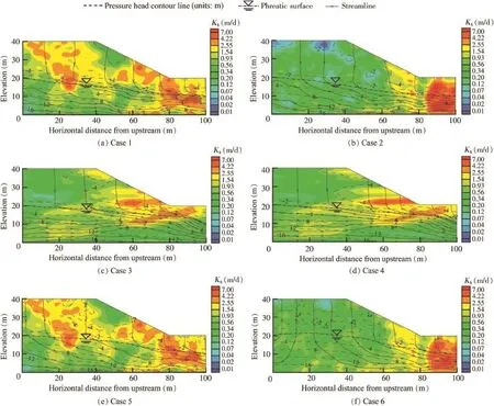
Fig.6.Spatial distributions of realized Ksfields and flow fields in steady state for different cases,subject to hydraulic scenario in which pressure head at slope toe reaches a minimum.

5.Conclusions

Results of the study show that,in an unsaturated region with a flux boundary,the dominant correlation between the pressure head P and saturated hydraulic conductivity Ksis negative and mainly occurs around the observation location of P.A location with a relatively high P is in a relatively low Kszone,while a location with a relatively low P is in a relatively high Kszone.The relatively low Kszones in the unsaturated region close to the slope surface are the more likely deformation and failure zones,which deserve special attention.We can further define the ratio of the vertical infiltration flux q to Ks(i.e.,q/Ks),with the vertical infiltration flux q set to be constant and uniform in this study.Therefore,P was positively correlated with q/Ksat the same location in the unsaturated region.Note that rainfall distribution is also important to the spatial distribution of P in unsaturated regions.If rainfall is non-uniform,the correlation between P and Ksbecomes more complex.However,P is still positively correlated with q/Ks.In addition,the position and shape of the phreatic surface may reveal the spatial distribution of Ksin a saturated region.That is,even if the vertical infiltration flux increases,the phreatic surface can remain low,depending on the distribution of Kswithin the heterogeneous hillslope.

The most likely spatial pattern of the Ksfield depends on the applied boundary conditions and factors,like the variance of lnKs,spatial structure anisotropy of lnKs,and vertical infiltration flux q.Overall,the spatial pattern obtained in this study can serve as a useful tool to quickly grasp the most likely distribution pattern of Kswithin a hillslope using observed pressure head fluctuations.Based on these findings, we conclude that,in terms of hillslope stability,heterogeneity causes some parts of the hillslope to be sensitive to externalhydraulic stimuli(e.g.,rainfall and reservoir level change)and other parts of the hillslope to be insensitive.This is due to the fact that heterogeneity affects the spatial distributions of the matric suction(i.e.,the absolute value of negative pore-water pressure),pressure head,and position and shape of the phreatic surface.This finding is essential since it explains why slopes with similar geometries would have different hydraulic or deformation responses to the same hydraulic stimuli.For example,some hillslopes are rainfall-sensitive while others are rainfall-insensitive in terms of hillslope stability.Research on these topics for hillslope stability analysis will be reported in future papers.

References

Bouwer,H.,1978.Groundwater Hydrology.McGraw-Hill College,New York.

Carsel,R.F.,Parrish,R.S.,1988.Developing joint probability distributions of soil water retention characteristics.Water Resour.Res.24(5),755-769. http://dx.doi.org/10.1029/WR024i005p00755.

Cho,S.E.,2012.Probabilistic analysis of seepage that considers the spatial variability of permeability for an embankment on soil foundation.Eng. Geol.133-134,30-39.http://dx.doi.org/10.1016/j.enggeo.2012.02.013.

Cho,S.E.,2014.Probabilistic stability analysis of rainfall-induced landslides considering spatial variability of permeability.Eng.Geol.171,11-20. http://dx.doi.org/10.1016/j.enggeo.2013.12.015.

Fenton,G.A.,Griffiths,D.V.,1993.Statistics of block conductivity through a simple bounded stochastic medium.Water Resour.Res.29(6),1825-1830. http://dx.doi.org/10.1029/93WR00412.

Gelhar,L.W.,1993.Stochastic Subsurface Hydrology.Prentice-Hall,Englewood Cliffs.

Griffiths,D.V.,Fenton,G.A.,1993.Seepage beneath water retaining structures founded on spatially random soil.G■eotechnique 43(4),577-587.http:// dx.doi.org/10.1680/geot.1993.43.4.577.

Griffiths,D.V.,Fenton,G.A.,2004.Probabilistic slope stability analysis by finite elements.J.Geotech.Geoenvironmental Eng.130(5),507-518. http://dx.doi.org/10.1061/(ASCE)1090-0241(2004)130:5(507).

Gui,S.,Zhang,R.,Turner,J.P.,Xue,X.,2000.Probabilistic slope stability analysis with stochastic soil hydraulic conductivity.J.Geotech.Geoenvironmental Eng.126(1),1-9.http://dx.doi.org/10.1061/(ASCE)1090-0241(2000)126:1(1).

Gutjahr,A.L.,1989.Fast Fourier Transforms for Random Field Generation: Project Report for Los Alamos Grant to New Mexico Tech.New Mexico Institute of Mining and Technology,Socorro.

Hughson,D.L.,Yeh,T.C.J.,2000.An inverse model for three-dimensional flow in variably saturated porous media.Water Resour.Res.36(4), 829-839.http://dx.doi.org/10.1029/2000WR900001.

Khaleel,R.,Freeman,E.J.,1995.Variability and Scaling of Hydraulic Properties for 200 Area Soils,Hanford Site.Westinghouse Hanford Company, Richland.

Li,B.,Yeh,T.C.J.,1998.Sensitivity and moment analyses of head in variably saturated regimes.Adv.Water Resour.21(6),477-485.http://dx.doi.org/ 10.1016/S0309-1708(97)00011-0.

Li,B.,Yeh,T.C.J.,1999.Cokriging estimation of the conductivity field under variably saturated flow conditions.Water Resour.Res.35(12),3663-3674. http://dx.doi.org/10.1029/1999WR900268.

Mao,D.,Wan,L.,Yeh,T.C.J.,Lee,C.,Hsu,K.,Wen,J.,Lu,W.,2011.A revisit of drawdown behavior during pumping in unconfined aquifers. Water Resour.Res.47(5).http://dx.doi.org/10.1029/2010WR009326.

Mualem,Y.,1976.A new model for predicting the hydraulic conductivity of unsaturated porous media.Water Resour.Res.12(3),513-522.http:// dx.doi.org/10.1029/WR012i003p00513.

Nielsen,D.R.,Biggar,J.W.,Erh,K.T.,1973.Spatial variability of fieldmeasured soil-waterproperties.Hilgardia 42(7),215-259.http:// dx.doi.org/10.3733/hilg.v42n07p215.

Rawls,W.J.,Brakensiek,D.L.,Saxtonn,K.E.,1982.Estimation of soil water properties.Trans.ASAE 25(5),1316-1320.http://dx.doi.org/10.13031/ 2013.33720.

Rulon,J.J.,Freeze,R.A.,1985.Multiple seepage faces on layered slopes and their implications for slope-stability analysis.Can.Geotech.J.22(3), 347-356.http://dx.doi.org/10.1139/t85-047.

Russo,D.,Bouton,M.,1992.Statistical analysis of spatial variability in unsaturated flow parameters.Water Resour.Res.28(7),1911-1925.http:// dx.doi.org/10.1029/92WR00669.

Russo,D.,1997.On the estimation of parameters of log-unsaturated conductivity covariance from solute transport data.Adv.Water Resour.20(4), 191-205.http://dx.doi.org/10.1016/S0309-1708(96)00019-X.

Santoso,A.M.,Phoon,K.K.,Quek,S.T.,2011.Effects of soil spatial variability on rainfall-induced landslides.Comput.Struct.89(11),893-900. http://dx.doi.org/10.1016/j.compstruc.2011.02.016.

Srivastava,A.,Babu,G.L.S.,Haldar,S.,2010.Influence of spatial variability of permeability property on steady state seepage flow and slope stability analysis. Eng. Geol. 110(3),93-101. http://dx.doi.org/10.1016/ j.enggeo.2009.11.006.

Sun,R.,Yeh,T.C.J.,Mao,D.,Jin,M.,Lu,W.,Hao,Y.,2013.A temporal sampling strategy for hydraulic tomography analysis.Water Resour.Res. 49(7),3881-3896.http://dx.doi.org/10.1002/wrcr.20337.

Sykes,J.F.,Wilson,J.L.,Andrews,R.W.,1985.Sensitivity analysis for steady state groundwater flow using adjoint operators.Water Resour.Res.21(3), 359-371.http://dx.doi.org/10.1029/WR021i003p00359.

U¨nlu¨,K.,Nielsen,D.R.,Biggar,J.W.,Morkoc,F.,1990.Statistical parameters characterizing the spatial variability of selected soil hydraulic properties. Soil Sci.Soc.Am.J.54(6),1537-1547.http://dx.doi.org/10.2136/ sssaj1990.03615995005400060005x.

van Genuchten,M.T.,1980.A closed-form equation for predicting the hydraulic conductivity of unsaturated soils.Soil Sci.Soc.Am.J.44(5), 892-898.http://dx.doi.org/10.2136/sssaj1980.03615995004400050002x.

White,I.,Sully,M.J.,1992.On the variability and use of the hydraulic conductivity alpha parameter in stochastic treatments of unsaturated flow. Water Resour. Res. 28(1),209-213. http://dx.doi.org/10.1029/ 91WR02198.

Wu,C.,Yeh,T.C.J.,Zhu,J.,Lee,T.H.,Hsu,N.,Chen,C.,Sancho,A.F.,2005. Traditional analysis of aquifer tests:Comparing apples to oranges？Water Resour.Res.41(9),W09402.http://dx.doi.org/10.1029/2004WR003717.

Yeh,T.C.J.,1992.Stochastic modelling of groundwater flow and solute transport in aquifers.Hydrol.Process 6(4),369-395.http://dx.doi.org/ 10.1002/hyp.3360060402.

Yeh,T.C.J.,Srivastava,R.,Guzman,A.,Harter,T.,1993.A numerical model for water flow and chemical transport in variably saturated porous media. Groundwater 31(4),634-644.http://dx.doi.org/10.1111/j.1745-6584. 1993.tb00597.x.

Yeh,T.C.J.,Mao,D.,Zha,Y.,Hsu,K.,Lee,C.,Wen,J.,Lu,W.,Yang,J.,2014. Why hydraulic tomography works？Groundwater 52(2),168-172.http:// dx.doi.org/10.1111/gwat.12129.

Yeh,T.C.J.,Khaleel,R.,Carroll,K.C.,2015.Flow Through Heterogeneous Geological Media.Cambridge University Press,Cambridge.

Zhang,J.,Yeh,T.C.J.,1997.An iterative geostatistical inverse method for steady flow in the vadose zone.Water Resour.Res.33(1),63-71.http:// dx.doi.org/10.1029/96WR02589.

Zhang,L.L.,Fredlund,D.G.,Zhang,L.M.,Tang,W.H.,2004.Numerical study of soil conditions under which can be maintained.Can.Geotech.J.41(4), 569-582.http://dx.doi.org/10.1139/t04-006.

Zhu,H.,Zhang,L.M.,Zhang,L.L.,Zhou,C.B.,2013.Two-dimensional probabilistic infiltration analysis with a spatially varying permeability function.Comput.Geotech.48,249-259.http://dx.doi.org/10.1016/ j.compgeo.2012.07.010.

This work was supported by the China Scholarship Council(Grant No. 201406410032),the National Natural Science Foundation of China(Grant No. 41172282),the Strategic Environmental Research and Development Program (Grant No.ER-1365),the Environmental Security and Technology Certification Program(Grant No.ER201212),and the National Science Foundation-Division of Earth Sciences(Grant No.1014594).

*Corresponding author.

E-mail address:yeh@hwr.arizona.edu(Tian-chyi Jim Yeh).

Peer review under responsibility of Hohai University.

http://dx.doi.org/10.1016/j.wse.2016.06.004

1674-2370/©2016 Hohai University.Production and hosting by Elsevier B.V.This is an open access article under the CC BY-NC-ND license(http:// creativecommons.org/licenses/by-nc-nd/4.0/).