A distributed Grid-Xinanjiang model with integration of subgrid variability of soil storage capacity

Wei-jian Guo*,Chuan-hai Wang,Teng-fei Ma,Xian-min Zeng,Hai Yang

aPowerChina Huadong Engineering Corporation Limited，Hangzhou 311122，China

bState Key Laboratory of Hydrology-Water Resources and Hydraulic Engineering，Hohai University，Nanjing 210098，China

cCollege of Hydrology and Water Resources，Hohai University，Nanjing 210098，China

Received 26 October 2015；accepted 15 March 2016

Available online 23 June 2016



A distributed Grid-Xinanjiang model with integration of subgrid variability of soil storage capacity

Wei-jian Guoa,*,Chuan-hai Wangb,c,Teng-fei Mab,c,Xian-min Zengb,c,Hai Yangb,c

aPowerChina Huadong Engineering Corporation Limited，Hangzhou 311122，China

bState Key Laboratory of Hydrology-Water Resources and Hydraulic Engineering，Hohai University，Nanjing 210098，China

cCollege of Hydrology and Water Resources，Hohai University，Nanjing 210098，China

Received 26 October 2015；accepted 15 March 2016

Available online 23 June 2016

Abstract

Realistic hydrological response is sensitive to the spatial variability of landscape properties.For a grid-based distributed rainfall-runoff model with a hypothesis of a uniform grid,the high-frequency information within a grid cell will be gradually lost as the resolution of the digital elevation model(DEM)grows coarser.Therefore,the performance of a hydrological model is usually scale-dependent.This study used the Grid-Xinanjiang(GXAJ)model as an example to investigate the effects of subgrid variability on hydrological response at different scales.With the aim of producing a more reasonable hydrological response and spatial description of the landscape properties,a new distributed rainfall-runoff model integrating the subgrid variability(the GXAJSV model)was developed.In this model,the topographic index is used as an auxiliary variable correlated with the soil storage capacity.The incomplete beta distribution is suggested for simulating the probability distribution of the soil storage capacity within the raster grid.The Yaogu Basin in China was selected for model calibration and validation at different spatial scales. Results demonstrated that the proposed model can effectively eliminate the scale dependence of the GXAJ model and produce a more reasonable hydrological response.

©2016 Hohai University.Production and hosting by Elsevier B.V.This is an open access article under the CC BY-NC-ND license(http:// creativecommons.org/licenses/by-nc-nd/4.0/).

Scale effect；Subgrid variability；Soil storage capacity；Incomplete beta distribution；GXAJSV model

1.Introduction

The advancement of geographic information system(GIS) and remote sensing(RS)in the last few decades has provided abundant spatial and temporal data for distributed rainfallrunoff modeling,such as the distribution of topography, soil,vegetation,and precipitation.However,more recent research suggests that with these data,distributed modeling approaches may not always provide improved simulations when compared to lumped conceptual models(Reed et al., 2004；Smith et al.,2004).In addition,the performance of a model can vary with the selected grid resolution.Part of the dilemma results from the uncertainty of model structure, parameter,and measurement.Another aspect is that the nonlinear hydrological processes are essentially sensitive to the spatial variability(Winchell et al.,1998；Smith et al., 2004).Most distributed rainfall-runoff models adopt the hypothesis of a uniform grid:the variability of the subgrid is ignored,and the variables and parameters are supposed to be constant within a grid cell.On the one hand,for most areas, information regarding heterogeneity at a small scale(less than 1000 m)is not monitored.On the other hand,even if the data are available,the model is also limited by the efficiencyof the numerical computation,especially if it is a macroscale model.The issues of how the variability of the hydrological variables(such as precipitation,infiltration,and evaporation) or hydrological parameters(such as hydraulic conductivity and roughness)at different spatial and temporal scales impacts the hydrological responses have been investigated by a number of researchers.For example,Singh(1997)surveyed the hydrological literature on the effect of spatial and temporal variability of hydrological factors on the stream flow hydrograph,and pointed out that the hydrological response is closely linked with storm dynamics.Bell and Moore(2000) investigated the sensitivity of catchment runoff models to rainfall using data from a dense rain gauge network and weather radar.Brocca et al.(2012)employed a statistical and temporal stability analysis to assess the spatial and temporal variability of the soil moisture at local and catchment scales. All these studies came to a conclusion that the sensitivity of a rainfall-runoff model to spatial and temporal variability is scale-dependent(Younger et al.,2009).

Different spatial modeling scales usually lead to different effective model parameters and hydrological responses.The issue is inherently linked with nonlinearity and heterogeneity of hydrological processes(Beven,2001).Under the hypothesis of a uniform grid,high-frequency information will be lost because the large sampling dimensions of the grids act as a filter(Band and Moore,1995；Kavvas,1999).Therefore,a reasonable discrete scale is critical for modeling the hydrological response.Wood et al.(1988)defined the hydrological response area as an areal element where the hydrological properties are not significantly different if a smaller scale of discretization is used.Kouwen et al.(1993)and Pietroniro and Soulis(2003)proposed the concept of grouped response units (GRUs)to group all the areas with a similar land cover type, and then summed the runoff from different groups of GRUs together and routed that amount of runoff to the river.A downscaling method is an alternative used to represent the subgrid variability.For example,Koster and Suarez(1999) depicted the general circulation model(GCM)grid square as a mosaic of vegetation tiles,with each tile consisting of a single vegetation type but without considering the physical location of each tile in the grid.Hahmann(2003)explicitly represented the spatial heterogeneities of the land surface with a subgrid imposed on each atmospheric grid.Famiglietti and Wood(1994)utilized a statistical-dynamical approach to simplify the large-scale modeling problem and aggregated the soil-vegetation-atmosphere transfer scheme(SVATS)to the macroscale.Moore(1985,2007)also highlighted the role of the probability distributed approach as a formulating principle in the development of rainfall-runoff model.

For the water cycle at a catchment scale,the distribution of soil moisture is a key control factor in partitioning the precipitation into evapotranspiration,surface runoff,interflow, and groundwater runoff(Wilson et al.,2005).The main feature of the Xinanjiang model,a widely used conceptual rainfall-runoff model for flood forecasting and simulation in humid and semi-humid regions of China,is that it adopts a power function to represent the variability of the soil storage capacity,WM,over a catchment(Zhao et al.,1995).This function has also been adopted by other hydrological models, e.g.,the variable infiltration capacity(VIC)model(Liang et al.,1996),the ARNO model(Todini,1996),the probability distributed model(PDM)(Moore,2007),and the grid-togrid(G2G)model(Moore et al.,2006).With the power function of WM,an analytical solution for the runoff generation can be obtained.However,this function lacks a theoretical basis.In the GXAJ model,a modified version of the Xinanjiang model,WM is derived from the soil texture and vegetation type(Liu et al.,2009；Yao et al.,2009),but is not easy to obtain at a fine resolution.In the G2G model,soil property data are used to determine WM at the model grid scale and a power function with terrain-slope dependence is used to represent its subgrid variability.

In this study we focused on the analysis of the spatial variability of WM at different spatial scales and its effect on the hydrological response.The GXAJ model was used to simulate the hydrological processes and assess the effects of the uniform grid on the catchment hydrological response.The GXAJSV model was developed with a subgrid parameterization scheme incorporated into the GXAJ model,aiming at partly eliminating the effect of scale on runoff generation.An attempt was made to construct the relationship between WM and the topographic index,TI.The proposed model was applied in the Yaogu Basin in China.The comparisons of the GXAJSV model with the GXAJ model are expected to provide further understanding of the effects of the subgrid variability on the hydrological response.

2.Model description

In this study,we adopted a similar model structure to the GXAJ model.For each grid,the main routines included evapotranspiration,runoff generation,and flow routing. Here,only a brief outline of evapotranspiration and flow routing is given.We mainly focus on the modeling of the runoff generation,taking account of the subgrid variability of WM.

2.1.Evapotranspiration

For each grid cell,the soil profile is divided into three layers:the upper,lower,and deeper layers.The layers correspond with evaporations of EU,EL,and ED,respectively；the water stored in each respective layer is WU,WL,and WD；and the maximum soil storage capacity in each respective layer is WUM,WLM,and WDM.Only when the layer above it runs out of water does evaporation from a layer occur.The total evaporation E equals the sum of EU,EL,and ED.

2.2.Runoff generation

The saturation excess mechanism was employed to model runoff generation and partitioning.In the original Xinanjiang model,the spatially uneven distribution of WM is depicted by a power function:

where WMmaxis the maximum watershed soil storage capacity,f/F is the fraction of the basin with a soil storage capacity less than WM,and B is the exponent.

The power function provides an analytical solution of runoff generation but lacks definite physical interpretation. Yao et al.(2009)utilized the soil texture and the land cover attributes to assign the WM value in each grid,and assumed it was spatially uniform within the grid cell.WM is dependent on the catchment topography,soil,and land cover types.For the measurement of soil properties,the conventional in situ measurements only provide finite point data.Remote sensing can describe the topography,surface soil,or vegetation properties of large areas,but it is characterized by a limited resolution.Therefore,these types of data are usually not accurate enough to provide the heterogeneity information at a small scale.To address this problem,two methods are commonly used.One method is interpolation on the spatial domain,for example by using Kriging,moving polynomials,and spline interpolation.Another method is to correlate the quantity of interest to an auxiliary variable whose spatial distribution can more readily be measured.The spatial distribution of the quantity is then inferred from the spatial distribution of the covariate(Bl¨oschl and Sivapalan,1995).In many previous studies,researchers have attempted to establish a relationship between the spatial and temporal distribution of soil properties and terrain indices,such as slope,wetness index,soil texture, and vegetation characteristics(Western et al.,1999；Schmidt and Hewitt,2004；Wilson et al.,2005；Cole and Moore, 2009).The relationship between TI and WM suggested by Sivapalan et al.(1997)is employed to determine the distribution of WM within the catchment.Although the influence of soil properties on the runoff generation is neglected in this simplified relationship,it has an advantage that WM can be expressed by TI,which can be more easily obtained at high resolution.A larger TI in a local area means less soil moisture deficit or easier runoff generation in response to rainfall input. On the contrary,a larger WM means a larger soil storage capacity in a local area,making runoff generation more difficult (Chen et al.,2007).Through the transformation,the normalized WM can be expressed by an index of relative difficulty of runoff generation(IRDG),calculated by

IRDG is transformed into WM by a linear transformation relationship:

where α and β are model parameters that quantify the WM value of a basin.

In the GXAJ model,the runoff only occurs when the soil moisture reaches saturation for each grid cell.Once soil reaches saturation,the runoff equals the rainfall excess without further loss.However,the high-frequency information will be smoothened as the uniform grid acts as a filter.Particularly for WM,due to the relatively short spatial correlation structure, the spatial distribution of WM is more easily affected by the smoothing effect(Western et al.,2004；Famiglietti et al., 2008).As a consequence,simulation of catchment hydrological response relies on the selection of grid resolution.For the scale-invariant hydrological response,it is necessary to take into account the subgrid variability of WM in the GXAJ model.Previous studies have recommended gamma,beta,or lognormal distributions to represent the soil characteristics (Kosugi,1996；Ryu and Famiglietti,2005).Therefore,we tested these three probability distribution functions to downscale the uniform soil storage capacity.As shown in Fig.1,the three curves of probability density functions(PDFs)can all fit well with the empirical statistical distribution of TI for the Yaogu Basin without any significant difference.The incomplete beta distribution,a generalization of the beta distribution, has the highest correlation coefficient among them,reaching 0.98.Besides that,as a bounded distribution,the beta distribution is more appropriate to describing the distribution of the normalized topographic index in a bounded domain.Although this statistical distribution of WM only represents the inter-grid variability,and the intra-grid variability is replaced by a mean value,it is reasonable to suppose that the statistical characteristics within the grid should follow the same distribution pattern as the inter-grid variability.Thus,the probability density function of the normalized topographic index within the grid can be written as

where︿TI is the normalized topographic index,Γ（·）is the gamma function,and a and b are two shape parameters.

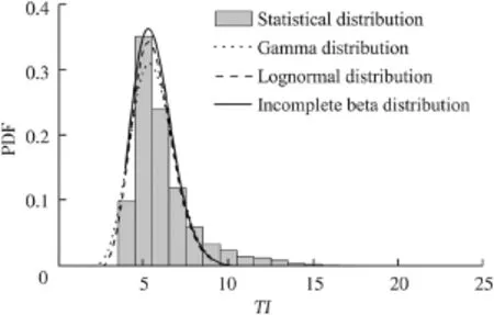
Fig.1.Comparison of curve fitting of three parametric probability distributions to empirical statistical distribution of topographic index for Yaogu Basin.

As a function of TI,the distribution of WM within the grid can also be derived numerically.The parameters of the incomplete beta distribution can be estimated by the mean and variance values of WM within the grid.We can obtain the mean value of WM of a grid cell using Eqs.(2)and(3).The variance indicates the fluctuation in WM within the grid cell,which can be derived by calibration against measured data.As shown in Fig.2,due to the antecedent soil moisture,part of the soil within the grid cell already reaches saturation.Influenced by the uneven distribution of WM within the grid,part of the net rainfall,Pe,is partitioned into the runoff R and the other part is stored in the soil ΔW.Therefore,we can estimate how much of the net rainfall Peis partitioned into runoff R by integration.The runoff R generated within the grid cell can be expressed as

where W0is the actual soil moisture,and IWMis the cumulative density function(CDF)of WM.

Depending on the free water capacity,the runoff is subdivided into three components,including surface runoff, interflow,and groundwater runoff.

2.3.Flow routing

For the daily simulation,the surface runoff is routed directly to the channel as the fast component.The interflow and groundwater runoff represent the slow component that is routed to the outlet of the corresponding subcatchment by two linear reservoirs with different lag times.The subcatchments are connected by the channel network.The outflow of each subcatchment is routed to the watershed outlet by the multiplereach Muskingum method.More details are available in Yao et al.(2009).

3.Field description and data

The Yaogu Basin,with a drainage area of about 1776 km2, was used to test the proposed distributed rainfall-runoff GXAJSV model.The Yaogu Basin is a sub-basin of the Xijiang Basin,located in southwestern China,and accounts for 70%of the area of the entire Xijiang Basin.The mainstream of the Xinxingjiang River originates in the Zhushan Mountain and flows into the Xijiang River at the Yaogu Station (26°14′N,109°37′E).It is 60.6 km in length,with a mean slope of 0.95% and an average annual water level and discharge of 12.33 m and 53.7 m3/s,respectively.The catchment is characterized by a humid climate with an average annual precipitation of about 1300-1700 mm.

Fig.2.Schematic representation of runoff generation within a grid.

The river network was extracted from the digital elevation model(DEM)provided by the U.S.Geological Survey (USGS)with a resolution of 90 m.The elevation of the catchment ranges from 11 to 1222 m.The DEM was then resampled to resolutions of 200 m,500 m,and 1000 m for the analysis of the effect of subgrid variability.By comparing to the actual river network,the river flow path was defined by a threshold of flow accumulation.We used the DEM to derive the slope,flow direction,flow length,and so on at different subgrid scales.The precipitation is monitored at nine rain gauging stations,including the Yaogu,Xinxing,Zhangtian, Gongcheng,Nansheng,Niancun,Chayuan,Lidong,and Tiantang stations(as shown in Fig.3).The precipitation was interpolated onto the model grid using the inverse distance squared method.The discharge gauging station is situated at Yaogu and records hourly discharge data.All the meteorological and hydrological data are available from 1999 to 2003 at the Yaogu Basin.

4.Results and discussion

4.1.Model calibration and validation

The calibration and validation of the model were performed using the hydrological data available from 1999 to 2003. Three flood events during this period were selected for analysis.Information for the three events is summarized in Table 1.To eliminate the influence of the initial condition,a run-in period of one month was used.

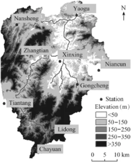
Fig.3.Location of gauging stations in study area.

Table 1Information of three flood events.

All the model parameters were calibrated based on the DEM with a resolution of 200 m.The results show a good correspondence between the simulated discharge and the measured data at the Yaogu Station.For all the three flood events,the Nash-Sutcliffe model efficiency(NSE)values of the flow hydrograph are all higher than 0.88.Also,the relative bias values at the flood peak(RB)are basically less than 0.02.

4.2.Influence of uniform grid on soil storage capacity curve and discharge

Within the saturation excess mechanism,WM is a key factor controlling the runoff generation.In order to test the influence of the resolution of the DEM on the spatial pattern of the soil storage capacity curve and its corresponding hydrological response,the DEMs with resolutions of 200 m,500 m, and 1000 m were derived by resampling the DEM with a resolution of 90 m.All tests were based on the original GXAJ model,in which the parameters and variables are considered uniform.Since the Xinanjiang model was developed,the realistic distribution of WM has not been strictly verified. Traditionally,WM is supposed to be correlated to the soil characteristics and the topography.In addition,the higher the data resolution,the more accurate the description of the spatial variability will be.Therefore,we adopted the spatial distribution of WM obtained using the DEM with a resolution of 90 m as the true value in this study.For comparison,the same parameters were chosen to transform TI into WM using Eqs.(2)and(3).Fig.4 shows the CDF of WM obtained at four DEM resolutions.A distinct shift in the mean value of WM can be observed as the grid size becomes finer.The mean value for the 1000-m grid size is approximately 73 mm,while it increases to 87 mm for the 90-m grid size.The total soil storage capacity of the catchment drops over 16%when the grid size increases from 90 m to 1000 m.

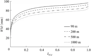
Fig.4.Distribution of soil storage capacity derived from different DEM scales.

The correlation coefficient of WM derived from different DEM resolutions was adopted to further evaluate the effect of grid scale on WM.Considering the WM value obtained using the DEM with the highest resolution(90 m)as the true value, we estimated the correlation coefficient of WM when the original DEM w…as aggregated into DEMs with resolutions of 180 m,270 m,,900 m.Fig.5 shows the average correlation coefficientbetween the true value and WM values obtained using DEMs at different grid scales.It is clear that the value has significantly deviated from the true value when the scale is aggregated in space,especially at the 900-m resolution,whenfalls below 0.5.It is evident that the distribution pattern of WM is sensitive to the spatial sampling resolution.

From the analysis described above,we can see the significant differences in the spatial distribution of WM resulting from the subgrid variability.The original GXAJ model was used to explore the scale effect on the hydrological response.As shown in Fig.6,for all the three flood events,the larger grid scale generally produces a larger peak discharge.In flood event 1,the peak discharge for the DEM with a resolution of 1000 m is 45%higher than for the DEM with a resolution of 200 m.The same situation also occurs in flood events 2 and 3.The respective peak discharges of flood events 2 and 3 for the DEM with a resolution of 1000 m are 93%and 23%higher than they were for the DEM with a resolution of 200 m.It is noteworthy that the simulated discharges for flood event 3 are highly coincident with one another at different grid scales,though a similar tendency still exists.This is because of the high-intensity precipitation of this event together with the wet antecedent soil moisture causing the soil moisture to reach saturation in a short period of time.Because of the saturation excess mechanism employed in the runoff generation,once the basin reaches saturation,all the precipitation will be converted into runoff without loss.Hence,the scale effect on runoff generation will gradually be eliminated.It is evident that the simulated discharge is sensitive to the spatial variability of the subgrid scale,especially for a small flood event.Compared with the low-resolution DEM,the high-resolution DEM actually enlarges the uneven distribution of WM,which leads to less runoff being generated and more water being stored in the soil.Therefore,for the same flood event,a larger model grid scale produces a higher flood peak discharge and a larger total flood volume.It can be concluded that the performance of the original GXAJ model is scale-dependent.This results from the differences of spatial variability at different scales. We usually think that higher resolutions produce better results. However,the selection of scale is limited by the efficiency ofthe numerical computation or data resolution in practice.It is not always feasible to run the model at a high resolution.

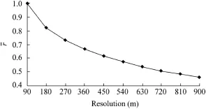
Fig.5.Average correlation coefficientof soil storage capacity between DEMs of original scale and other scales.

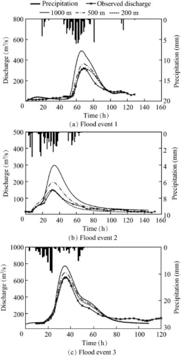
Fig.6.Comparison of scale effect on hydrological response of GXAJ model for three flood events.

4.3.Analysis for GXAJSV model with integration of subgrid variability

Based on the concept of an effective model parameter,the model can be used at different scales by calibrating the effective model parameters against the measured data,with no need to change the model structure.However,this will result in scale dependence of the model parameters,which may cause inconvenience for model application to ungauged basins.Therefore,the aim of the proposed GXAJSV model is to eliminate the scale effect on the hydrological response.On the basis of the GXAJ model,we incorporated the subgrid variability of WM.The incomplete beta distribution was adopted to replace the original uniform grid at the subgrid scale and TI was used as the auxiliary variable to be correlated with WM. To evaluate the performance of the GXAJSV model,comparisons were made with the GXAJ model.All the parameters of the GXAJSV model were kept consistent with the GXAJ model at different scales.

We first examined the effects on the spatial pattern of the curve of WM.Fig.7 shows the comparisons of CDFs derived directly from the DEMs with resolutions of 200 m,500 m,and 1000 m and the one incorporating the subgrid variability of WM.The DEM with a resolution of 90 m was still used as the true value to assess the performance of the subgrid parameterization method.

As shown in Fig.7,the proposed method successfully downscales WM.Compared to the curve of WM with the hypothesis of a uniform grid,the curves incorporating the variability with the incomplete beta distribution of WM at a subgrid scale fit better to the one from the 90-m scale.The mean value of WM shows a distinct shift when the subgrid variability is taken into account.The variance of WM in one grid increases with the grid size and,therefore,the difference between two curves obtained by consideration and without consideration of the subgrid variability is greater for a coarser DEM than for a finer one.

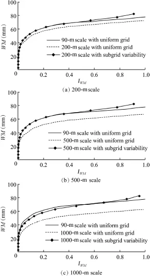
Fig.7.Comparison of soil storage capacity curves from DEMs at different scales with uniform grid and subgrid variability.

Table 2Comparison of model performance of GXAJ and GXAJSV models at different DEM resolutions.

Previous studies have demonstrated that the simulated discharge is sensitive to the DEM resolution.We expect that the incorporation of the subgrid variability can provide a scaleinvariant hydrological response.Table 2 compares the performance of the GXAJ and GXAJSV models in the three flood events.The model efficiency of flow hydrograph and relative bias of peak discharge were used as two criteria to evaluate the model performance.

Compared to the GXAJ model,the performance of the GXAJSV model at all the scales is much better.In the simulation of flood event 1,the model efficiency values for the GXAJ model are 0.94,0.84,and 0.67 for the DEMs with resolutions of 200 m,500 m,and 1000 m,respectively. Meanwhile,for the GXAJSV model,the corresponding model efficiency values reach 0.94,0.90,and 0.89.A similar trend can also be found in the other two flood events.For the relative bias of the flood peak,the average bias values of the GXAJ model for the three scales are 0.03,0.21,and 0.56 for the three flood events.However,they decrease to 0.01,0.03,and 0.04 for the GXAJSV model.From the comparisons described above,it is evident that incorporation of the subgrid variability of WM in the GXAJSV model can effectively eliminate the scale dependence of the hydrological response.Since the subgrid variability is taken into account,the spatial variability of the watershed at different scales can generally remain consistent.

To further investigate the performance of the GXAJ and GXAJSV models for the long-term simulation,we examined the water balance of the Yaogu Basin in 1999 at a daily time step.The initial soil moisture was considered dry(with a relative soil content θ of 0.2).The simulated annual runoff values for the GXAJ model are 546 mm,550 mm,and 552 mm at DEM resolutions of 200 m,500 m,and 1000 m, respectively.As in a single flood event,the runoff for annual simulation increases with grid scale.Meanwhile,for the GXAJSV model,the total runoffs are 545 mm,545 mm,and 546 mm,respectively.It is obvious that the bias in simulated runoff at different scales significantly decreases when the subgrid variability of WM is incorporated.

Fig.8 depicts the spatial distribution of the difference in the long-term runoff obtained by the two models at different scales.It is noted that a significant difference in runoff generation mainly occurs in hillslope areas.The patterns are similar at all scales.This is because the riparian areas are always associated with relatively low values of WM,which easily reaches saturation.As mentioned above,once the soil reaches saturation,the scale effect on runoff generation will no longer exist.Meanwhile,for the hillslope areas that have larger WM values,no runoff will be generated when the total net rainfall is less than WM in the GXAJ model.For the GXAJSV model,due to the uneven distribution of WM within the grid cell,the runoff may already be generated before the soil in the grid cell fully reaches saturation.Thus,for areas that have large WM values,a difference in the long-term runoff will gradually appear.

5.Conclusions

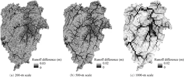
Fig.8.Difference in runoff generation between GXAJ and GXAJSV models at different scales.

In this study,we used the GXAJ model as an example to investigate the sensitivity of a distributed hydrological model to scale.Analysis of the Yaogu Basin shows that the peak discharge and flood volume vary with the DEM resolution. Both the peak discharge and flood volume are overestimatedat large scales.With the uniform grid hypothesis,model performance is scale-dependent,with the difference across scales also depending on antecedent soil conditions and rainfall intensity.Because of the saturation excess mechanism employed by the GXAJ model,once the soil reaches saturation,the scale effect on runoff generation will gradually be eliminated.

To achieve a scale-invariant hydrological response,this paper proposed an improved version,the GXAJSV model,that incorporates the subgrid variability of the soil storage capacity WM.The differences between the GXAJ and GXAJSV models are attributed to two treatments:(1)in the GXAJSV model,the derivation of WM is based on the topographic index TI,rather than soil or vegetation data,and the relationship between TI and WM is constructed to obtain information about soil properties,because the high-resolution TI is much easier to obtain directly from DEM data；and(2)the incomplete beta distribution is used to describe the subgrid variability of WM. The analysis shows that the incomplete beta distribution provides a best fit for the inter-grid spatial pattern of WM. Furthermore,we assumed that the inter-grid and intra-grid variability would follow the same probability distribution for a certain variable.Therefore,the incomplete beta distribution was adopted to replace the uniform distribution of WM at the subgrid scale.

The performance of the GXAJSV model was compared with the original GXAJ model for three flood events and the annual water balance.The results show that the proposed method successfully downscales WM at different scales.The soil storage capacity curves from the coarser DEMs(with resolutions of 200 m,500 m,and 1000 m)can fit better to that from the original DEM(with a resolution of 90 m)when the subgrid variability is incorporated.Moreover,the GXAJSV model can also effectively eliminate the difference in the model performance at different scales.Analysis of the scale effect on flow routing is a subject for further research.

References

Band,L.E.,Moore,I.D.,1995.Scale:Landscape attributes and geographical information systems.Hydrol.Process.9(3-4),401-422.http://dx.doi.org/ 10.1002/hyp.3360090312.

Bell,V.A.,Moore,R.J.,2000.The sensitivity of catchment runoff models to rainfall data at different spatial scales.Hydrol.Earth Syst.Sci.Discuss. 4(4),653-667.http://dx.doi.org/10.5194/hess-4-653-2000.

Beven,K.,2001.How far can we go in distributed hydrological modelling？Hydrol.Earth Syst.Sci.5(1),1-12.http://dx.doi.org/10.5194/hess-5-1-2001.

Bl¨oschl,G.,Sivapalan,M.,1995.Scale issues in hydrological modelling:A review.Hydrol.Process.9(3-4),251-290.http://dx.doi.org/10.1002/ hyp.3360090305.

Brocca,L.,Tullo,T.,Melone,F.,Moramarco,T.,Morbidelli,R.,2012. Catchment scale soil moisture spatial-temporal variability.J.Hydrol. 422-423,63-75.http://dx.doi.org/10.1016/j.jhydrol.2011.12.039.

Chen,X.,Chen,Y.D.,Xu,C.Y.,2007.A distributed monthly hydrological model for integrating spatial variations of basin topography and rainfall. Hydrol.Process.21(2),242-252.http://dx.doi.org/10.1002/hyp.6187.

Cole,S.J.,Moore,R.J.,2009.Distributed hydrological modelling using weather radar in gauged and ungauged basins.Adv.Water Resour.32(7), 1107-1120.http://dx.doi.org/10.1016/j.advwatres.2009.01.006.

Famiglietti,J.S.,Wood,E.F.,1994.Multiscale modeling of spatially variable waterand energy balanceprocesses.WaterResour.Res.30(11), 3061-3078.http://dx.doi.org/10.1029/94WR01498.

Famiglietti,J.S.,Ryu,D.,Berg,A.A.,Rodell,M.,Jackson,T.J.,2008.Field observations of soil moisture variability across scales.Water Resour.Res. 44(1).http://dx.doi.org/10.1029/2006wr005804.

Hahmann,A.N.,2003.Representing spatial subgrid-scale precipitation variability in a GCM.J.Hydrometeorol.4(5),891-900.http://dx.doi.org/ 10.1175/1525-7541(2003)004＜0891:RSSPVI＞2.0.CO；2.

Kavvas,M.L.,1999.On the coarse-graining of hydrologic processes with increasing scales.J.Hydrol.217(3-4),191-202.http://dx.doi.org/ 10.1016/S0022-1694(98)00252-2.

Koster,R.D.,Suarez,M.J.,1999.A simple framework for examining the interannualvariabilityoflandsurfacemoisturefluxes.J.Clim.12(7),1911-1917. http://dx.doi.org/10.1175/1520-0442(1999)012＜1911:ASFFET＞2.0.CO；2.

Kosugi,K.,1996.Lognormal distribution model for unsaturated soil hydraulic properties.Water Resour.Res.32(9),2697-2703.http://dx.doi.org/ 10.1029/96WR01776.

Kouwen,N.,Soulis,E.,Pietroniro,A.,Donald,J.,Harrington,R.,1993. Grouped response units for distributed hydrologic modeling.J.Water Resour.Plan.Manag.119(3),289-305.http://dx.doi.org/10.1061/(ASCE) 0733-9496(1993)119:3(289).

Liang,X.,Lettenmaier,D.P.,Wood,E.F.,1996.One-dimensional statistical dynamic representation of subgrid spatial variability of precipitation in the two-layer variable infiltration capacity model.J.Geophys.Res.101(D16), 21403-21422.http://dx.doi.org/10.1029/96jd01448.

Liu,J.,Chen,X.,Zhang,J.,Flury,M.,2009.Coupling the Xinanjiang model to a kinematic flow model based on digital drainage networks for flood forecasting.Hydrol.Process.23(9),1337-1348.http://dx.doi.org/10.1002/ hyp.7255.

Moore,R.J.,1985.The probability-distributed principle and runoff production at point and basin scales.Hydrol.Sci.J.30(2),273-297.http://dx.doi.org/ 10.1080/02626668509490989.

Moore,R.J.,Cole,S.J.,Bell,V.A.,Jones,D.A.,2006.Issues in flood forecasting:Ungauged basins,extreme floods and uncertainty.In: Tchiguirinskaia,J.,Thein,K.N.N.,Hubert,P.,eds.,Frontiers in Flood Research.IAHS Publication,Paris,pp.103-122.

Moore,R.J.,2007.The PDM rainfall-runoff model.Hydrol.Earth Syst.Sci. Discuss.11(1),483-499.http://dx.doi.org/10.5194/hess-11-483-2007.

Pietroniro,A.,Soulis,E.D.,2003.A hydrology modelling framework for the Mackenzie GEWEX programme.Hydrol.Process.17(3),673-676.http:// dx.doi.org/10.1002/hyp.5104.

Reed,S.,Koren,V.,Smith,M.,Zhang,Z.,Moreda,F.,Seo,D.-J.,DMIP participants,2004.Overalldistributedmodelintercomparisonprojectresults.J. Hydrol.298(1-4),27-60.http://dx.doi.org/10.1016/j.jhydrol.2004.03.031.

Ryu,D.,Famiglietti,J.S.,2005.Characterization of footprint-scale surface soil moisture variability using Gaussian and beta distribution functions during the Southern Great Plains 1997(SGP97)hydrology experiment.Water Resour.Res.41(12).http://dx.doi.org/10.1029/2004wr003835.

Schmidt,J.,Hewitt,A.,2004.Fuzzy land element classification from DTMs based on geometry and terrain position.Geoderma 121(3-4),243-256. http://dx.doi.org/10.1016/j.geoderma.2003.10.008.

Singh,V.P.,1997.Effect of spatial and temporal variability in rainfall and watershed characteristics on stream flow hydrograph.Hydrol.Process. 11(12),1649-1669.http://dx.doi.org/10.1002/(SICI)1099-1085(19971015) 11:12＜1649::AID-HYP495＞3.0.CO；2-1.

Sivapalan,M.,Woods,R.A.,Kalma,J.D.,1997.Variable bucket representation of TOPMODEL and investigation of the effects of rainfall heterogeneity. Hydrol.Process.11(9),1307-1330.http://dx.doi.org/10.1002/(SICI)1099-1085(199707)11:9＜1307::AID-HYP562＞3.0.CO；2-Y.

Smith,M.B.,Koren,V.I.,Zhang,Z.,Reed,S.M.,Pan,J.J.,Moreda,F.,2004. Runoff response to spatial variability in precipitation:An analysis of observed data.J.Hydrol.298(1-4),267-286.http://dx.doi.org/10.1016/ j.jhydrol.2004.03.039.

Todini,E.,1996.The ARNO rainfall-runoff model.J.Hydrol.175(1-4), 339-382.http://dx.doi.org/10.1016/S0022-1694(96)80016-3.

Western,A.W.,Grayson,R.B.,Bl¨oschl,G.,Willgoose,G.R.,McMahon,T.A., 1999.Observed spatial organization of soil moisture and its relation toterrain indices.Water Resour.Res.35(3),797-810.http://dx.doi.org/ 10.1029/1998WR900065.

Western,A.W.,Zhou,S.L.,Grayson,R.B.,McMahon,T.A.,Bl¨oschl,G., Wilson,D.J.,2004.Spatial correlation of soil moisture in small catchments and its relationship to dominant spatial hydrological processes.J.Hydrol. 286(1-4),113-134.http://dx.doi.org/10.1016/j.jhydrol.2003.09.014.

Wilson,D.J.,Western,A.W.,Grayson,R.B.,2005.A terrain and data-based method for generating the spatial distribution of soil moisture.Adv.Water Resour.28(1),43-54.http://dx.doi.org/10.1016/j.advwatres.2004.09.007.

Winchell,M.,Gupta,H.V.,Sorooshian,S.,1998.On the simulation of infiltration-and saturation-excess runoff using radar-based rainfall estimates: Effects of algorithm uncertainty and pixel aggregation.Water Resour.Res. 34(10),2655-2670.http://dx.doi.org/10.1029/98wr02009.

Wood,E.F.,Sivapalan,M.,Beven,K.,Band,L.,1988.Effects of spatial variability and scale with implications to hydrologic modeling.J.Hydrol. 102(1-4),29-47.http://dx.doi.org/10.1016/0022-1694(88)90090-X.

Yao,C.,Li,Z.,Bao,H.,Yu,Z.,2009.ApplicationofadevelopedGrid-Xinanjiang model to Chinese watersheds for flood forecasting purpose.J.Hydrol.Eng. 14(9),923-934.http://dx.doi.org/10.1061/(ASCE)HE.1943-5584.0000067.

Younger,P.M.,Freer,J.E.,Beven,K.J.,2009.Detecting the effects of spatial variability of rainfall on hydrological modelling within an uncertainty analysis framework.Hydrol.Process.23(14),1988-2003.http:// dx.doi.org/10.1002/hyp.7341.

Zhao,R.,Liu,X.,Singh,V.,1995.The Xinanjiang model.In:Singh,V.P.,ed., Computer Models of Watershed Hydrology.Water Resources Publications, pp.215-232.

This work was supported by the Graduate Students Scientific Research Innovation Plan of Jiangsu Province(Grant No.CXZZ12_0243),the China Scholarship Council(Grant No.201306710013),the State Major Project of Water Pollution Control and Management(Grant No.2014ZX07101-011),and the Special Fund for Public Welfare of Ministry of Water Resources of China (Grant No.201501007).

*Corresponding author.

E-mail address:gjjsher@126.com(Wei-jian Guo).

Peer review under responsibility of Hohai University.

http://dx.doi.org/10.1016/j.wse.2016.06.003

1674-2370/© 2016 Hohai University.Production and hosting by Elsevier B.V.This is an open access article under the CC BY-NC-ND license(http:// creativecommons.org/licenses/by-nc-nd/4.0/).