A Mean-variance Problem in the Constant Elasticity of Variance（CEV）Model

Hou Ying-lianD Liu Guo-xin

（1.College of Mathematics and Information Science，Hebei Normal University，Shijiazhuang，050024）

（2.School of Science，Hebei University of Technology，Tianjin，300401）

（3.Department of Mathematics and Physics，Shijiazhuang Tiedao University，Shijiazhuang，050043）

Communicated by Jiang Chun-lan

A Mean-variance Problem in the Constant Elasticity of Variance（CEV）Model

Hou Ying-li1anD Liu Guo-xin2，3

（1.College of Mathematics and Information Science，Hebei Normal University，Shijiazhuang，050024）

（2.School of Science，Hebei University of Technology，Tianjin，300401）

（3.Department of Mathematics and Physics，Shijiazhuang Tiedao University，Shijiazhuang，050043）

Communicated by Jiang Chun-lan

In this paper，we focus on a constant elasticity of variance（CEV）model and want to find its optimal strategies for a mean-variance problem under two constrained controls：reinsurance/new business and investment（no-shorting）.First，a Lagrange multiplier is introduced to simplify the mean-variance problem and the corresponding Hamilton-Jacobi-Bellman（HJB）equation is established.Via a power transformation technique and variable change method，the optimal strategies with the Lagrange multiplier are obtained.Final，based on the Lagrange duality theorem，the optimal strategies and optimal value for the original problem（i.e.，the efficient strategies and efficient frontier）are derived explicitly.

constant elasticity of variance model，mean-variance，optimal strategy

2010 MR subject classification：49J20，60J60

Document code：A

Article ID：1674-5647（2015）03-0242-11

1　Introduction

In this paper，we study a constant elasticity of variance（CEV）model.The CEV model is an extension model of the geometric Brownian motion（GBM）.It was developed by［1-2］，and then it was usually applied to calculating the option pricing problems（see［3-7］）.In recent years，the CEV model began to apply in optimal investment research（see［8-10］）.

The study of mean-variance portfolio selection model should date back to Markowitz's Nobel Prize-winning work（see［11］）.In this paper，we introduce the dynamic mean-variance problem to the CEV model.And the aim is to get the optimal strategy of this problem under two constrained controls：reinsurance/new business and investment（no-shorting）as stated by Bai and Zhang［12］.They studied the mean-variance problem under two types of risk models：a classical model and its diffusion approximation.They constructed a continuously differentiable function to get a viscosity solution and gave a verification theorem.Because of the appearance of the constant elasticity of variance，the approach to construct a viscosity solution cannot be used in our model.Fortunately，via the power transformation technique and variable change method proposed by Cox［4］，we obtain the optimal strategy with the Lagrange multiplier for our model.And we can find the Theorem 2.2 in［12］is just our case when the constant elasticity of variance is zero.Finally，based on the Lagrange duality theorem in［13］，the optimal strategy and optimal value for the original problem（i.e.，the efficient strategy and efficient frontier）are derived explicitly.

The rest of this paper is organized as follows.Section 2 presents the CEV model which we focus on.In Section 3，the optimization problem is developed.We get the optimal strategy in Section 4 and find the efficient strategy and efficient frontier in Section 5.

2　The Model

Let the claim process be denoted by

where a and b are positive constants，W0（t）is a standard Brownian motion.Assume that the premium is c0=（1+η）a with safety loading η＞0.

Let u（t）≥0 denote the retention level of reinsurance/new business（u（t）∈［0，1］corresponded to a proportional reinsurance and u（t）＞1 corresponded to acquiring new business）. The insurer pays reinsurance premium at the rate c1=（1+θ）a（1-u（t））with safety loading θ＞η＞0.So the surplus process is given by the dynamics

In addition，the insurer is supposed to invest its surplus in a risk-free asset（bond or bank account）and a risky asset.Let S0（t）denote the price process of the risk-free asset given by

Let S1（t）denote the price process of the risky asset described by a CEV model

where r1＞r0is the expected instantaneous rate of the risky asset，σ）is the instantaneous volatility and β≤0 is the elasticity parameter.｛W0（t））：t≥0｝and｛W1（t））：t≥0｝are standard Brownian motions defined on a complete probability space（Ω，F，P）.The filtration F=｛Ft｝is right continuous filtration of sigma-algebras on this space and denotesthe information structure generated by Brownian motion.The processes｛W0（t））：t≥0｝and｛W1（t））：t≥0｝are assumed to be independent.

A strategy π is described by a two-dimensional dynamic process（u（t），l（t）），where u（t）denotes the retention level of reinsurance/new business at time t，l（t）denotes the proportion invested in the risky asset at time t.Here，short-selling is prohibited，i.e.，l（t）≥0.Let X（t）represent the resulting surplus process after incorporating strategy π into（2.2）.The dynamics of X（t）can be preserved as follows：

A strategy π is said to be admissible when it is adapted to｛Ft｝and satisfies the borrowing or lending capability of the insurer.Denote the set of all admissible strategies by Π.

3　Optimization Problem

The purpose is to find an admissible strategy such that the expected terminal wealth satisfies

while the risk measured by the variance of the terminal wealth

is minimized.It is reasonable to assume that

which coincides with the amount that the insurer would earn if none of the initial wealth invested in the risky asset.And the above problem can be stated as the following optimization problem：

In the above problem，the equality constrain E［X（T）］=d can be dealt with by introducing a Lagrange multiplier 2δ∈R and letting d′=d-δ.For every fixed δ，the problem can be solved via the following optimal stochastic control problem：

In the sense that the two problems have exactly the same optimal strategy.Now，we let

Our goal is to find the optimal value function

and the optimal strategy π∗=（u∗（t），l∗（t））such that

To solve the above problem，we use the dynamic programming approach described in［14］. From standard arguments，we get the following Hamilton-Jacobi-Bellman（HJB）equation about the optimization problem：

with V（T，s，x）=（x-d′）2.

The first order minimizing conditions for the optimal strategies u∗and l∗are

We obtain

Putting（3.5）in（3.3），we obtain a partial differential equation（PDE）for the function V

with V（T，s，x）=（x-d′）2.

Now the problem is to solve（3.6）for the function V and replace it in（3.5）in order to obtain the optimal strategies.

4　Optimal Strategies

We conjecture a solution to（3.6）with the following form

where

Then

Putting these derivatives in（3.6），we have

Transform the above formula into the following form

Let the coefficients of（x-c）and g be zero.Then

Taking into account the boundary condition c（T）=d′，the solution to（4.3）is

Noting that（4.4）is a nonlinear second-order PDE，it is very difficult to find an explicit solution.So we can use power transformation and variable change technique proposed in［4］in the derivation of the CEV option price to transform the nonlinear equation into a linear one.Let

with the boundary condition f（T，y）=1.Then

Substituting these derivatives into（4.4），we get the following PDE

We want to find a solution to（4.7）with the following form

with the boundary conditions

Putting this into（4.7），we obtain

We decompose（4.9）into two parts for eliminating the dependence in y and t

（1）For β=0，it is easy to get

And from（3.5），we can get

When x≥c（t），we have u∗≤0 and l∗≤0 in（4.12）.At this time，we can put u∗=0 and l∗=0.This result can be stated as follows：

Theorem 4.1If β=0，then the optimal strategy for insurer is

Theorem 4.1 coincides with the Theorem 2.2 in［12］.

（2）For β＜0，the solutio ns to（4.10）and（4.11）can be divided into three cases.

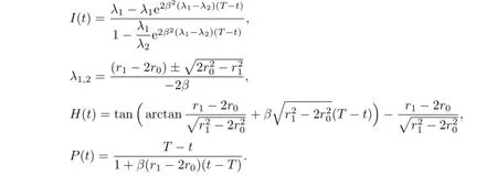
where

where

where

From above calculations，we have

where

Thus l∗can be transformed as

where

The following Lemma is obtained.

Lemma 4.1For any r1＞r0，we have N（0）≤N（t）≤1.

Proof.Recall that

and

Thus，

This shows that N（t）is an increasing function on［0，T］，and N（T）=1，so N（0）≤N（t）≤1.

Thus，for any r1＞r0，we have N（0）≤N（t）≤1.

If N（0）≥0，then N（t）≥0；if N（0）＜0，then there exists a t0such that N（t0）=0，N（t）＜0 for 0＜t＜t0，and 0＜N（t）＜1 for t0＜t＜T.

From the above calculations，we obtain

Theorem 4.2The optimal strategy with the Lagrange multiplier for the insurer is as follows：

（1）If x≥c（t），N（0）≥0，or N（0）＜0 and t≥t0，then（u∗，l∗）=（0，0）；

（2）If x≥c（t），N（0）＜0 and t＜t0，then

（3）If x＜c（t），N（0）≥0，or N（0）＜0 and t≥t0，then

（4）If x＜c（t），N（0）＜0 and t＜t0，then

5　Efficient Strategy and Efficient Frontier

In this section，we apply the results established in Section 4 to the mean-variance problem.

Let t=0 in（4.1）.Then（4.1）can be translated into the following function：

The value still depends on δ.To obtain the minimum value of Var（X（T）），we just need to maximize V（0，S1（0），X（0））-δ2over δ according to the Lagrange duality theorem in［13］.

（1）For β=0，we have

V（0，S1（0），X（0））-δ2

A simple calculation shows that（5.2）attains its maximum value

at

Under the assumption

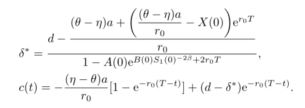
stated in Section 3，we have δ∗＜0.Summarizing the above results，we have

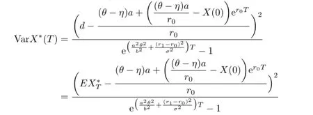
Theorem 5.1When β=0，the efficient frontier and the efficient strategy corresponding to the expected terminal wealth EX∗（T）=d are

and

where

（2）For β＜0，we have

V（0，S1（0），X（0））-δ2

where

and

Based on the assumption

we can derive the maximum value

at

Then the following theorem is obtained.

Theorem 5.2When β＜0，the efficient frontier and the efficient strategy corresponding to the expected terminal wealth EX∗（T）=d are

（1）if X∗（t）≥c（t），N（0）≥0，or N（0）＜0 and t≥t0，then

（2）if X∗（t）≥c（t），N（0）＜0 and t＜t0，then

（3）if X∗（t）＜c（t），N（0）≥0，or N（0）＜0 and t≥t0，then

（4）if X∗（t）＜c（t），N（0）＜0 and t＜t0，then

where

References

［1］Cox J C.Notes on Option Pricing I：Constant Elasticity of Variance Diffusions.Stanford：Stanford University，1975，unpublished manuscript.

［2］Cox J C，Ross S A.The valuation of options for alternative stochastic processes.J.Financ. Econ.，1976，4：145-166.

［3］Bechers S.The constant elasticity of variance model and its implications for option pricing.J. Financ.，1980，35（3）：661-673.

［4］Cox J C.The constant elasticity of variance option pricing model.J.Portfolio Manag.，1996，22：16-17.

［5］Davydov D，Linetsky V.The valuation and hedging of barrier and lookback option under the CEV process.Manag.Sci.，2001，47：949-965.

［6］Detemple J，Tian W D.The valuation of American options for a class of diffusion processes. Manag.Sci.，2002，48：917-937.

［7］Lo C F，Yuen P H，Hui C H.Constant elasticity of variance option pricing model with timedependent parameters.Int.J.Theory Appl.Finance，2000，3：661-674.

［8］Gao J.Optimal portfolios for DC pension plans under a CEV model.Insur.Math.Econ.，2009，44：479-490.

［9］Xiao J W，Hong Z，Qin C L.The constant elasticity of variance（CEV）model and the legendre transform-dualsolution for annuity contracts.Insur.Math.Econ.，2007，40：302-310.

［10］Gu M D，Yang Y P，Li S D，Zhang J Y.Constant elasticity of variance model for proportional reinsurance and investment strategies.Insur.Math.Econ.，2010，46：580-587.

［11］Markowitz H.Portfolio selection.J.Finance，1952，7：77-91.

［12］Bai L H，Zhang H Y.Dynamic mean-variance with constrained risk control for the insurer. Math.Methods Oper.Res.，2008，68（1）：181-205.

［13］Luenberger D G.Optimization by Vector Space Methods.New York：Wiley，1969.

［14］Fleming W H，Soner H M.Controlled Markov Process and Viscosity Solutions.Berlin-New York：Springer，1993.

10.13447/j.1674-5647.2015.03.06

date：Oct.1，2013.

The NSF（11201111）of China，Hebei Province Colleges and Universities Science，and Technology Research Project（ZD20131017）.

E-mail address：houyingli@gmail.com（Hou Y L）.