Analysis of a multi-patch dynamical model about cattle brucellosis
Juan Zhang, Shigui Ruan, Guiquan Sun,Xiangdong Sun, Zhen Jin
(1.School of Mechatronic Engineering, North University of China, Taiyuan, Shan′xi 030051, China;2.Complex Systems Research Center, Shanxi University, Taiyuan, Shan′xi 030006, China;3.Department of Mathematics, University of Miami, Coral Gables, FL 33124-4250,USA;4.School of Mathematical Science, Fudan University, Shanghai 200433, China;5.The Laboratory of Animal Epidemiological Surveillance, China Animal Health & Epidemiology Center, Qingdao, Shandong 266032, China)
1 Introduction
Brucella, one of the world′s major zoonotic pathogens known,causes infectious abortion in animals and Malta Fever in man[1]. Since many kinds of domestic animals,such as sheep, cattle, dogs, pig and so on, can be infected by brucella,brucellosis usually causes economic devastation on a global scale. China is no exception. In Zhejiang province which locates in the southern China, the livestock breeding, dairy, the leather processing industry have gotten great development.A mass of dairy cows, beefs, row fur and other animal by-products were taken to trade annually. But it has also brought lots of cattle brucellosis infection[2, 3]. In fact, the cow remains an intermittent carrier for years in China[4]. For cattle, transmission of brucella typically occurs through direct contact with brucella carriers or oral contact with aborted foetal material including the bacteria throughout the byre[4, 5]. Bull can spread infection through semen, but often the disease leads to infertility or arthritis. More detailed information about cattle brucellosis can be seen in [6].
Since Brucellosis caused by brucella is a non-fatal disease, it is often overlooked by the majority of the scientific community. The local government of Zhejiang province has regularly taken detection measures and culled infected cattle immediately. Yet, the data of positive cattle brucellosis in Zhejiang are rising year by year and it has influenced the local economy, even leads to the local prevalence of human brucellosis. From Fig.1, we can see that brucellosis has been spreading from north to south in Zhejiang province.So, one of main reasons of the geographical spread of the disease is the transportation of cattle between cities within Zhejiang province. Cattle transportation can cause cross infection of individuals among different regions. Besides, through vehicles and staff movement, it can also lead to the disperdal of brucella surviving in environment.Therefore, public health officials and scientific community should pay more attention to the transmission of cattle brucellosis.
Dynamical systems method is one of the most useful and important tools in studying biological and epidemiological models[7-13].Some researches have applied dynamical systems method to study brucellosis[14-17].In 1994,Gonzalez-Guzman and Naulin[14]were the first to apply dynamical models to study bovine brucellosis.In 2005,besides transmission within sheep and cattle populations, Zinsstag et al.[17]considered the transmission to humans in a dynamical model. The livestock are classified into three subclasses: the susceptible, the seropositive and the immunized. In 2009, Xie and Horan[15]built a simple dynamical model with the susceptible, the infected and the resistant subclasses to discuss brucellosis in the elk and cattle population. In 2010, Ainseba et al.[16]considered two transmission modes about the ovine brucellosis in their model: direct mode caused by infected individuals and indirect mode related to brucella in the environment. For the transmission of brucellosis in China, there are also some studies[18-22]. Hou et al.[20]investigated the transmission dynamics of sheep brucellosis in Inner Mongolia Autonomous Region of China. Zhang et al.[21]and Nie et al.[22]established dynamical models about dairy cattle brucellosis in Zhejiang and Jilin Provinces, respectively. According to the spatial spread of disease, there are two types of model we can apply:multi-patch models[23-30]and reaction-diffusion models[31-33].The goal of this paper is to establish an n-patch dynamical model to discuss the effects of cattle dispersal and brucella diffusion on the geographical spread of the disease.
The article is organized as follows. In Sections 2 , we propose ann-patch model about cattle brucellosis with cattle transportation and brucella diffusion, and analyze its dynamical behavior. In section 3, we apply numerical method to discuss the transmission of the disease between two patches under different conditions. In section 4, we give a brief discussion.
2 Model and dynamical behavior
There are 11 cities in Zhejiang province, where Hangzhou is the provincial capital. More generally, we propose an epidemic dynamical model with cattle dispersal betweennpatches. The number of cattle in each patch can be denoted byNi,i=1,2,…,n. For each patch, the cattle population is divided into three classes:

Fig.1 The distribution of infected dairy cattle in Zhejiang from 2001 to 2010.(a) 2001. (b)2002. (c)2003. (d) 2004. (e)2005. (f)2006.(g) 2007. (h)2008. (i)2009.(j) 2010.
susceptible,exposed and infective individuals, the numbers of which at timetinith patch are denoted bySi(t),Ei(t) andIi(t), respectively. During the infected period, the infected individuals (the exposed and the infectious individuals) discharge brucella into the environment. The quantity of brucella in environment is denoted byVi(t). Consequently, the susceptible cattle can be infected by contacting with the exposed cattle, the infectious cattle and the brucella in environment. Compared with the infectious individuals, the transmission coefficient of the exposed individuals is relatively smaller. So the auxiliary parameterθis introduced. The internal relationship of each individual innpatches can be described in the following system and the parameter meanings can be seen in Table 1, where parametersAi,βi,αi,mi,δi,μi,riandwiare all positive constants.θis a parameter whose value is between 0 and 1.aji,bji,cjianddji(j≠i) are non-negative constants.aii,bii,ciianddiiare non-positive constants.
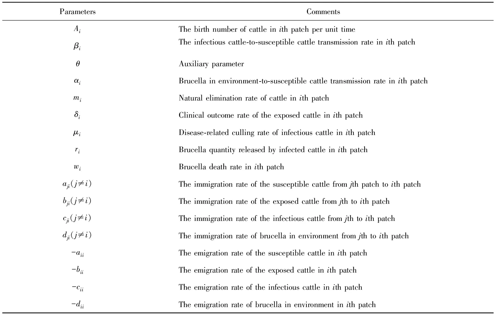
(1)
It is easy to know that there exist the following relationships for the migration rates.
∀ 1≤i≤n.
(2)
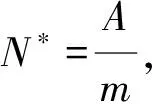
Firstly, we consider the existence and uniqueness of the disease-free equilibrium. Let the right hand side of system (1) be zero and chooseEi=Ii=Vi=0, we can obtain the following system.
which can be expanded as follows.
Observing the coefficient matrix and combining Eq.(2), we know that the coefficient matrix is absolutely diagonally dominant about columns. So the above system has a unique untrivial solution and the solution is positive. Thus the corresponding disease-free equilibrium of system (1) is existent and unique, which can be denoted as
E0=(S10,0,0,0,…,Si0,0,0,0,…,Sn0,0,0,0).
Applying the next generation matrix method, we can present the expression of the basic reproduction number.Define
and
where,
and
The basic reproduction number isR0=ρ(FV-1). DefiningM=F-Vands(M):=max{Reλ:λis an eigenvalue ofM}, we have the following result.
Lemma2There hold two equivalences[34]:
R0<1⟺s(M)<0,R0>1⟺s(M)>0.
(3)
By Theorem 2 in [34], the disease-free equilibriumE0is locally asymptotically stable whenR0<1 and unstable whenR0>1. Now we further investigate the global dynamical behavior ofE0.
Firstly, we consider the auxiliary system
(4)
whose Jacobian matrix is
It is already known that the Jacobian matrix is absolutely diagonally dominant about column and the system (3) has a unique positive equilibriumS0=(S10,S20,S30,…,Sn0)T. Moreover, -mi+aii<0, 1≤i≤n. So, all eigenvalues of the Jacobian matrix have negative real parts which imply thatS0is locally stable. Since system (4) is a linear system, equilibriumS0is globally stable.
Theorem1WhenR0<1, the disease-free equilibriumE0of system (1) is globally asymptotically stable inΓ.
ProofNow, we only need to prove the global attraction of the disease-free equilibrium. BecauseR0<1, thens(M)<0. For small enoughη,s(M+Mη)<0, where
It is obvious to know that
(5)
Then the following auxiliary system is introduced.
(6)
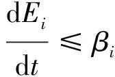
The positive equilibriumS0of system (6) has been proved to be globally stable. So, forη, there existsTsuch that ∀t>T,S(t)≤S0+η, whereS(t)=(S1(t),…,Sn(t)). Thus, we obtain the following system.


Define
X={(S1,E1,I1,V1,…,Sn,En,In,Vn):Si≥0,Ei≥0,Ii≥0,Vi≥0,i=1,…,n},
X0={(S1,E1,I1,V1,…,Sn,En,In,Vn)∈X:Ei>0,Ii>0,Vi>0,i=1,…,n},
∂X0=XX0.
Considering the auxiliary system
(7)
For system (7), similar as system (4), there exists a unique positive equilibriumS0() and it is global asymptotically stable. By the implicity function theorem, it follows thatS0() is continuous in term of. For givenτ, we can restrictsmall enough such thatS0()≥S0-τfor allt>T1.
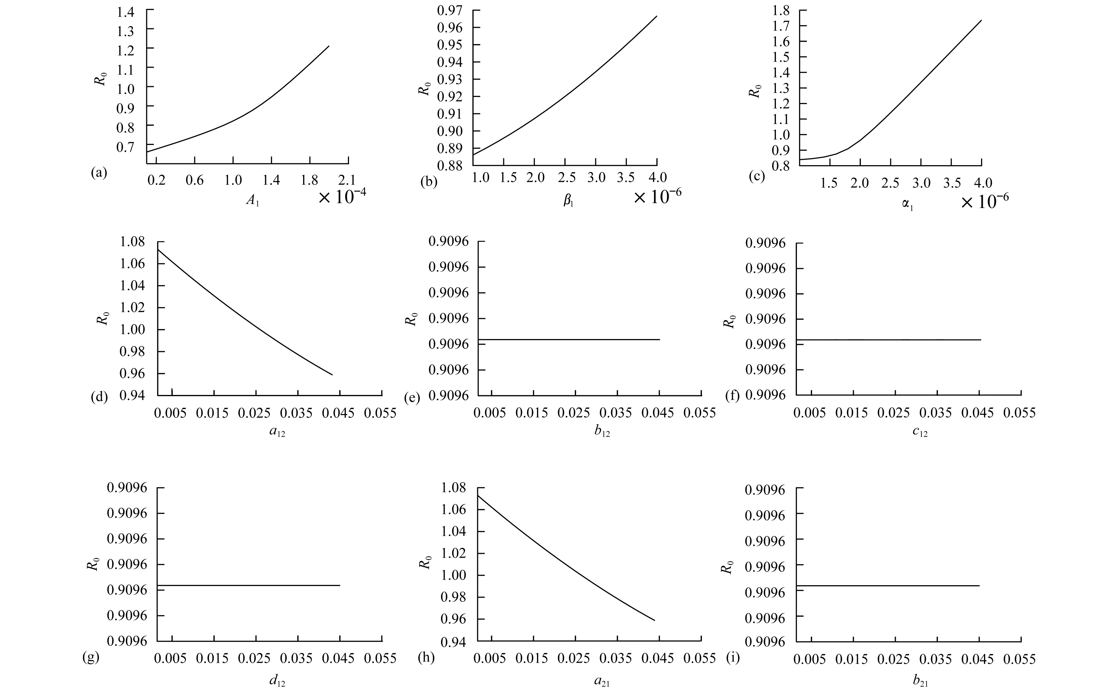
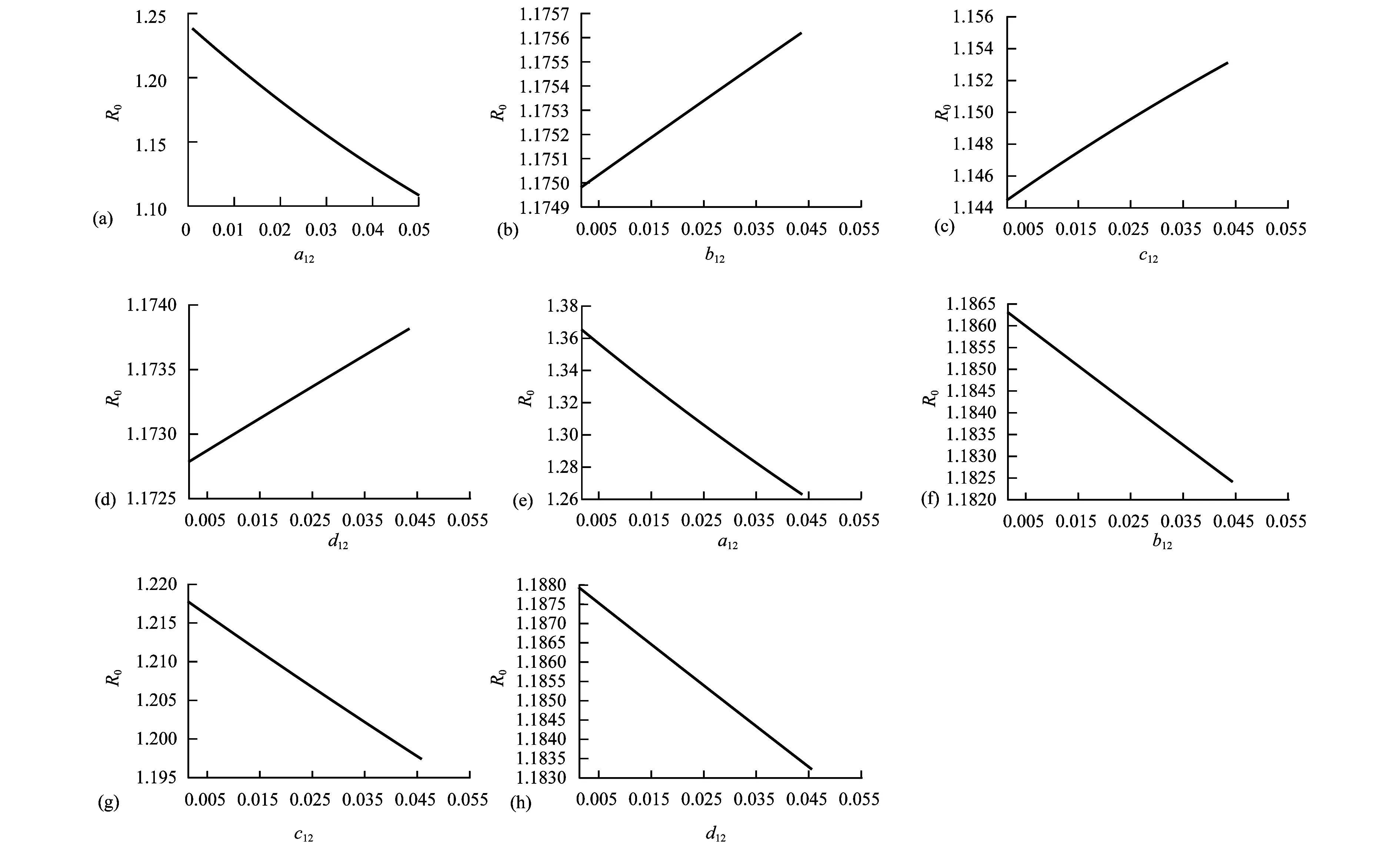
Theorem2WhenR0>1, there exists positive constantsuch that when ‖(Ei(0),Ii(0),Vi(0))‖ (8) ProofBecauseR0>1,s(M)>0. So, for small enoughτ,s(M-Mτ)>0, where Now we proceed by contradiction to prove the above conclusion. Suppose, there existandT>0 such thatEi(t)<,Ii(t) (9) For the right side system, there exists a unique positive equilibriumS0() which is global asymptotically stable. There exists a large enoughT1>Tsuch thatS(t)≥S0(). BecauseS0()≥S0-τ,S(t)≥S0-τfor allt>T1. Thus, there holds Becauses(M-Mτ)>0,Ii(t)→∞,Ei(t)→∞,Vi(t)→∞ ast→∞,i=1…n, which is a contraction. So, inequality (8) is well-founded. Theorem3WhenR0>1, system (1) admits at least one positive equilibrium, and there exists positive constantsuch that every solution of (1) with (Si(0),Ei(0),Ii(0),Vi(0))∈X0satisfies (10) ProofFirstly, we show that system (1) is uniformly persistent with respect to (X0,∂X0). It is easy to know that bothXandX0are positively invariant and ∂X0is relatively closed inX. Moreover, from Lemma 1, system (1) is point dissipative. SetM∂={(S(0),E(0),I(0),V(0)):(S(t),E(t),I(t),V(t))∈∂X0, ∀t≥0,i=1,…,n}, whereS(t)=(S1(t),…,Sn(t)),E(t)=(E1(t),…,En(t)),I(t)=(I1(t),…,In(t)),V(t)=(V1(t),…,Vn(t)). It is needed to show that M∂={(S(t),0,…,0):S(t)≥0}. (11) Noting that {(S(t),0,…,0):S(t)≥0}⊆M∂, (12) we only need to prove M∂⊆{(S(t),0,…,0):S(t)≥0,i=1,…,n}. (13) Suppose not. Assume (S(0),E(0),I(0),V(0))∈M∂. There exist ani0(1≤i0≤n) and at0such that (Ei0(t0),Ii0(t0),Vi0(t0))T>0. Then we can separate {1,…,n} into two setsQ1andQ2such that (Ei(t0),Ii(t0),Vi(t0))T=0, ∀i∈Q1, (Ei(t0),Ii(t0),Vi(t0))T>0, ∀i∈Q2. It is easy to know thatQ1andQ2are not empty. Fori∈Q2, without loss of generality, we assumeEi(t0)>0,Ii(t0)=Vi(t0)=0. From the equationsIi′(t0)=δiEi(t0)>0 andVi′(t0)=riEi(t0)>0, we can know that there is a small enough0>0 such thatEi(t)>0,Ii(t)>0,Vi(t)>0,i∈Q2fort0 In this section, for simplicity, assumingn=2, we perform numerical simulation to study the effects of cattle dispersal on brucellosis transmission. Leta12=-a22,a21=-a11,b12=-b22,b21=-b11,c12=-c22,c21=-c11,d12=-d22,d21=-d11. Then system (1) reduces to (14) Also, we can obtain the basic reproduction numbersR1,R2of two patches under the situation that there exists no migration of cattle and the diffusion of brucella between them as follows. Now, we mainly have a look at the effect of some parameters and population scales on the basic reproduction number and the number of the infected individuals, respectively. Example1When all the parameter values are same between two patches and the dispersal rates of each subpopulation from one patch to the other are taken as the same. Assume thatA1=A2=13000;m1=m2=0.25;δ1=δ2=6;μ1=μ2=0.85;r1=r2=5;w1=w2=6;a12=a21=b12=b21=c12=c21=d12=d21=0.1;β1=β2=2.1×10⁻⁶;θ=0.5. (1) Ifα1=α2=2.2×10⁻⁵,R0=R1=R2=1.0886. In this case, the brucellosis in two patches will become endemic with time (see Fig.2). (2) Ifα1=α2=1.8×10⁻⁵,R0=R1=R2=0.9096. In this case, the infectious cattle in two patches will disappear with time (see Fig.3). Fig.2 The number of the infectious cattle with time. (a) in the first patch. (b) in the second patch. The initial values will be taken as S1(0)=40000,E1(0)=7,I1(0)=12,V1(0)=100,S2(0)=40000,E2(0)=I2(0)=V2(0)=0. Fig.3 The number of the infectious cattle with time. (a) in the first patch. (b) in the second patch.S1(0)=40000,E1(0)=7,I1(0)=12,V1(0)=100,S2(0)=40000,E2(0)=I2(0)=V2(0)=0. Figs.2 and 3 confirm that the basic reproduction numberR0is the transmission threshold of brucellosis in two patches. Besides, the sensitivity of the basic reproduction numberR0in term ofβ1,α1,A1,a12,b12,c12,d12can be seen in Fig.4. From Fig.4, we know thatR0will increase with the increase ofA1. Comparing withβ1, the effect ofα1onR0is larger. What is interesting is that the transport of susceptible cattle can reduceR0, which implies that the dispersal of susceptible cattle can relief the transmission situation of brucellosis in the whole region. However, the transport of the infected cattle or the diffusion of brucella has no influence onR0. Example2When the numbers of cattle in two patches are different, the disease situation will be different from Example 1.Assume that the number of cattle in the first patch is larger than the second patch.A1=20000;A2=10000;m1=m2=0.25;δ1=δ2=6;μ1=μ2=0.85;r1=r2=5;w1=w2=6;β1=β2=2.1×10⁻⁶;θ=0.5;α1=α2=2.2×10⁻⁵. (1) If the dispersal rate of the first patch is smaller than the second patch,a12=b12=c12=d12=0.3,a21=b21=c21=d21=0.1. In this case,R0=1.1785,R1=1.3993,R2=0.6997(see Fig.5). (2) If the dispersal rate of the first patch is larger than the second patch,a12=b12=c12=d12=0.1,a21=b21=c21=d21=0.3. In this case,R0=1.4059,R1=1.3993,R2=0.6997(see Fig.6). From Figs. 5 and 6, we can see that the patch whose dispersal rate is bigger, the number of infectious cattle will be smaller. For the patch that has larger cattle population, the emigration of susceptible cattle can reduceR0, see Fig.7. However, the emigration of the brucella carriers and the diffusion of brucella can increaseR0. For the patch that has smaller cattle population, the emigration of all subpopulation can reduceR0. Fig.4 R0 in term of parameters A1,β1,α1,a12,b12,c12,d12,a21,b21. Fig.5 The number of the infectious cattle with time. (a) in the first patch. (b) in the second patch. The initial values will be taken as S1(0)=40000,E1(0)=7,I1(0)=12,V1(0)=100,S2(0)=20000,E2(0)=I2(0)=V2(0)=0. Example3We need to know that when the basic reproduction numbersR1andR2of two patches are both less than 1, what is aboutR0? The parameter values are the same as Example 2 except forα1andα2. Assumeα1=α2=1.8×10⁻⁵. (1) If the dispersal rate of the first patch is larger than the second patch,a12=b12=c12=d12=0.3,a21=b21=c21=d21=0.1. In this case,R0=0.9548,R1=0.9096,R2=0.6997. The brucellosis in two patches will disappear with time. (see Fig.8) (2) If the dispersal rate of the first patch is larger than the second patch,a12=b12=c12=d12=0.1,a21=b21=c21=d21=0.3. In this case,R0=1.0233,R1=0.9096,R2=0.6997. The infectious disease in two patches will become endemic with time.(see Fig.9) Fig.6 The number of the infectious cattle with time. (a) in the first patch. (b) in the second patch. The initial values will be taken as S1(0)=40000,E1(0)=7,I1(0)=12,V1(0)=100,S2(0)=20000,E2(0)=I2(0)=V2(0)=0. Fig.7 R0 in term of parameters a12,b12,c12,d12,a21,b21,c21,d21. Fig.8 The number of the infectious cattle with time. (a) in the first patch. (b) in the second patch. The initial values will be taken as S1(0)=40000,E1(0)=7,I1(0)=12,V1(0)=100,S2(0)=20000,E2(0)=I2(0)=V2(0)=0. Fig.9 The number of the infectious cattle with time. (a) in the first patch. (b) in the second patch. The initial values will be taken as S1(0)=40000,E1(0)=7,I1(0)=12,V1(0)=100,S2(0)=20000,E2(0)=I2(0)=V2(0)=0. From Figs. 8 and 9, we can see that if the basic reproduction numbers of two patches without cattle and brucella dispersal are less than 1, with the change of dispersal rates between patches, the basic reproduction number in the whole region will be variable. It can be less than 1, also can be more than 1 as the dispersal rates increase. For Zhejiang province of China, the recent prevalance of brucellosis in cattle is believed to be caused by the transportation of cattle and brucella between cities in Zhejiang province. In this article, we applied ann-patch dynamical model to study the effect of dispersal of cattle and brucella on the spatial transmission of brucellosis. Firstly, we analyzed the dynamical behavior of the model. More specifically, assumingn=2, we carried out the sensitivity analysis of the basic reproduction number and the number of the infectious cattle in term of different parameter values. Finally, it is obtained that the dispersal of the susceptible cattle can relief the spread of brucellosis in the whole region. However, the emigration of the brucella carriers or the diffusion of brucella in patch whose rasing quantity of cattle is larger can increaseR0. On the contrary, the emigration of the brucella carriers or the diffusion of brucella in patches where the amount of live cattle is smaller can reduceR0. In summary, the dispersal of the susceptible population of each patch and the centralization of the infected cattle to the patches where the breeding scale is bigger are in favor of the controlling of the disease. : [1] M. L. Boschiroli,V. Foulongne,D.O′Callaghan.Brucellosis:a worldwide zoonosis[J].Current Opinion in Microbiology,2001,4:58-64. [2] W. M. Xu,S. F. Shi,Y. Yang,H. Y. Jin,H. Wang.Epidemic situation and exploration of the prevention and control strategies on Brucellosis in Zhejiang Province[J].Chinese Rural Health Service Administration,2007,27(3):209-211. [3] W. M. Xu,H. Wang,S. J. Zhu,Y. Yang,J. Wang,X. Y. Jin,L. L. Gao,Y. Yang.2000-2007 the human and livestock brucellosis situation and control measure in Zhejiang province[J].Chin. J. Prev. Med.,2009,43(8):746-747. [4] Z. Bercovich.Maintenance of Brucella abortus-free herds:a review with emphasis on the epidemiology and the problems in diagnosing Brucellosis in areas of low prevalence[J].Vet. Quart.,1998,20:81-88. [5] D. C. Blood,O. M. Radostits.Veterinary medicine:A textbook of the diseases of cattle,sheep,pigs,goats,horses.(7th ed.)[M].London:Balliere Tindall,1989. [6] T. England,L. Kelly,R. D. Jones, A. Macmillan, M. Wooldridge.A simulation model of brucellosis spread in British cattle under several testing regimes[J].Prev. Vet. Med.,2004,63:63-73. [7] J. Zhang,Z. Jin,G. Q. Sun,S. G. Ruan.Spatial spread of rabies in China[J].J. Appl. Analy. Compu.,2012,2(1):111-126. [8] J. Q. Li,X. C. Song,F. Y. Gao.Global stability of a virus infection model with two delays and two types of target cells[J].J. Appl. Analy. Compu.,2012,2(3),281-292. [9] K. Hong,P. X. Weng.Stability and traveling waves of diffusive predator-prey model with age-structure and nonlocal effect[J].J Appl. Analy. Compu.,2012,2(2):173-192. [10] J. Zhang,Z. Jin,G. Q. Sun,T. Zhou,S. G. Ruan.Analysis of rabies in China:Transmission dynamics and control[J].PLoS one,2011,6(7):e20891. [11] J. Zhang,Z. Jin,G. Q. Sun,X. D. Sun,S. G. Ruan.Modeling seasonal rabies epidemic in China[J].Bull. Math. Biol.,2012,74:1226-1251. [12] J. Zhang,Z. Jin,G. Q. Sun,X. D. Sun,Y. M. Wang,B. X. Huang.Determination of original infection source of H7N9 avian influenza by dynamical model[J].Scientific Reports,2014,4:4846. [13] M. T. Li,G. Q. Sun,J. Zhang,Z. Jin.Global dynamic behavior of a multigroup cholera model with indirect transmission[J].Discrete Dynamics in Nature and Society,2013,Article ID 703826. [14] J. Gonzalez-Guzman,R. Naulin.Analysis of a model of bovine brucellosis using singular perturbations[J].J. Math. Biol.,1994,33:211-223. [15] X. Fang,D. H. Richard.Disease and behavioral dynamics for brucellosis control in greater yellowstone area[J].J. Agr. Resour. Ec.,2009,34(1):11-33. [16] B. Ainseba,C. Benosman,P. Magal.A model for ovine brucellosis incorporating direct and indirect transmission[J].J. Biol. Dynam.,2010,4(1):2-11. [17] J. Zinsstag,F. Roth,D. Orkhon,G. Chimed-Ochir,M. Nansalmaa,J. Kolar,P. Vounatsou.A model of animal-human brucellosis transmission in Mongolia[J].Prev. Vet. Med.,2005,69:77-95. [18] M. T. Li,G. Q. Sun,Y. F. Wu,J. Zhang,Z. Jin.Transmission dynamics of a multi-group brucellosis model with mixed cross infection in public farm[J].Applied Mathematics and Computation,2014,237(5):582-594. [19] M. T. Li,G.Q. Sun,J. Zhang,Z. Jin,X. D. Sun,Y. M. Wang,B. X. Huang,Y. H. Zheng.Transmission dynamics and control for a Brucellosis model in Hinggan league of Inner Mongolia,China[J].Mathematical Bioscience and Engineering,(Accepted),2014. [20] Q. Hou,X. D. Sun,J. Zhang,Y. J. Liu,Y. M. Wang, Z. Jin.Modeling the transmission dynamics of sheep brucellosis in Inner Mongolia Autonomous Region,China[J].Math. Biosci.,2013,242:51-58. [21] J. Zhang,X. D. Sun,G. Q. Sun,Q. Hou,M. T. Li,B. X Huang,Z. Jin.Prediction and control of brucellosis transmission of dairy cattle in Zhejiang Province,China[M].In press. [22] J. Nie,X. D. Sun,G. Q. Sun,J. Zhang, Z. Jin.Modeling the transmission dynamics of dairy cattle brucellosis in Jilin Province,China[M].In press. [23] D. Z. Gao,S. G. Ruan.A multipatch malaria model with logistic growth populations[J].SIAM J. Appl. Math.,2012,72(3):819-841. [24] W. D. Wang,X. Q. Zhao.An epidemic model in a patchy environment[J].Math. Biosci.,2004,190:97-112. [25] D. Z. Gao,S. G. Ruan.An SIS patch model with variable transmission coefficients[J].Math. Biosci.,2011,232:110-115. [26] F. Zhang,X. Q. Zhao.A periodic epidemic model in a patchy environment[J].J. Math. Anal. Appl.,2007,325:496-516. [27] P. Auger,E. Kouokam,G. Sallet,M. Tchuente,B. Tsanou.The Ross-Macdonald model in a patchy environment[J].Math. Biosci.,2008,216:123-131. [28] E. Kouokam,P. Auger,H. Hbid,M. Tchuente.Effect of the number of patches in a multi-patch SIRS model with fast migration on the basic reproduction rate[J].Acta. Biotheor.,2008,56:75-86. [29] W. D. Wang,X. Q. Zhao.An epidemic model with population dispersal and infection period[J].SIAM J. Appl. Math.,2006,66(4):1454-1472. [30] L. J. S. Allen,B. M. Bolker,Y. Lou,A. L. Nevai.Asymptotic profiles of the steady states for an SIS epidemic patch model[J].SIAM J. Appl. Math.,2007,67:1283-1309. [31] Y. Morita.Spectrum comparison for a conserved reaction-diffusion system with a variational property[J].J. Appl. Analy. Compu.,2012,2(1):57-71. [32] H. S. Mahato,M. Böhm.Global existence and uniqueness of solution for a system of semilinear diffusion-reaction equations[J].J. Appl. Analy. Compu.,2012,3(4),357-376. [33] L. Z. Li,N. Li,Y. Y. Liu,L. H. Zhang.Existence and uniqueness of a traveling wave front of a model equation in synaptically coupled neuronal networks[J].J. Appl. Analy. Compu.,2013,3(2),145-167. [34] P. Van Den Driessche ,J. Watmough.Reproduction numbers and sub-threshold endemic equilibria for compartmental models of disease transmission[J].Math. Biosci.,2002,180(1-2):29-48. [35] H. Thieme.Convergence results and a Poincaré-Bendixson trichotomy for asymptotically au-tonomous differential equations[J].J. Math. Biol.,1992,30:755-763. [36] W. M. Hirsch,H. L. Smith,X. Q. Zhao.Chain transitivity attractivity and strong repellors for semidynamical systems[J].J. Dynam. Differ. Equat.,2001,13(1):107-131. [37] H. R. Thieme.Persistence under relaxed point-dissipativity (with application to an endemic model)[J].SIAM J. Math. Anal.,1993,24:407-435. [38] X. Q. Zhao.Uniform persistence and periodic coexistence states in infinite-dimensional periodic semiflows with applications[J].Can. Appl. Math. Quart.,1995,3:473-495.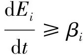

3 Application to two patches






4 Discussion

