Analysis of a Prey-predator Model with Disease in Prey∗

LI JIAN-JUN,GAO WEN-JIEAND SUN PENG

(1.College of Science,Liaoning Technical University,Fuxin,Liaoning,123000)

(2.Institute of Mathematics,Jilin University,Changchun,130012)

Analysis of a Prey-predator Model with Disease in Prey∗

LI JIAN-JUN1,GAO WEN-JIE2AND SUN PENG2

(1.College of Science,Liaoning Technical University,Fuxin,Liaoning,123000)

(2.Institute of Mathematics,Jilin University,Changchun,130012)

In this paper,a system of reaction-di ff usion equations arising in ecoepidemiological systems is investigated.The equations model a situation in which a predator species and a prey species inhabit the same bounded region and the predator only eats the prey with transmissible diseases.Local stability of the constant positive solution is considered.A number of existence and non-existence results about the nonconstant steady states of a reaction di ff usion system are given.It is proved that if the di ff usion coefficient of the prey with disease is treated as a bifurcation parameter, non-constant positive steady-state solutions may bifurcate from the constant steadystate solution under some conditions.

eco-epidemiology,bifurcation,non-constant positive steady solution

1 Introduction

Mathematical ecology and mathematical epidemiology are major fields of study.Since transmissible disease in ecological situation cannot be ignored,it is very important from both the ecological and the mathematical points of view to study ecological systems subject to epidemiological factors.A number of studies have been performed in this direction;see[1]–[9] and the references therein.Combining a typical SI model with an open system of variable size and a general predator-prey model,Bairagi et al.proposed a eco-epidemiological model in[10]as follows:

where u,v and w are the densities of susceptible prey,infected prey and predator,respectively;r,k,mi,i=1,2,···,5 are positive constants;m1is the rate of transmission;m2is the search rate;m3is the death rate of infected prey;m4represents the conversion factor; m5is the total death of predator population and a is the half saturation coefficient.

This model implies that the prey is divided into two disjoint classes,susceptible prey u and infected prey v.Only susceptible prey has capability of reproducing,but the infected prey still contributes with u to population growth towards the carrying capacity k.Disease transmission follows the simple law of mass action.The disease is spread among the prey population only.The infected population do not recover or become immune.It is assumed that predator consume only infected preys at the rates m2v/(a+v).For more detailed biological meaning the reader may consult[10].

As we know,most of the eco-epidemiological models are ODE systems.If we take into account the distribution of the species in spatial locations within a fixed bounded domainΩ∈RNwith smooth boundary∂Ωand both species di ff use,i.e.,move from points of high to points of low population density,then(1.1)may be rewritten as

where∂nis the outward directional derivative normal to∂Ωand the positive constants d1, d2and d3are the di ff usion rates.The initial data u(x,0),v(x,0)and w(x,0)are continuous functions on.The homogeneous Neumann boundary condition means that(1.2)is selfcontained and has no population fl ux across the boundary∂Ω.

The positive steady state solutions of(1.2)satisfy the following elliptic system:

For the simplicity of notation,we denote

We note that(1.2)has a unique nonnegative global solution U which can be proved by using the method of upper and lower solutions.In addition,if u(x,0)0,v(x,0)0,w(x,0)0, then the solution is positive,i.e.,u＞0,v＞0,w＞0 onfor all t＞0.The equation(1.2)

and hence(1.3)has a constant positive solution U0=(u0,v0,w0),where

Hereafter,we always suppose that(1.5)holds if there is no special demonstrativeness.

There are many works on the existence of positive steady states of ecological models. For predator-prey models,see[11]–[15]and the references therein.The general form of a weakly-coupled parabolic equation

was discussed by Brown[16],where the asymptotic stability of critical points was given.

The main aim of this paper is to study the local stability of positive constant steady solution as well as the non-existence of non-constant positive steady state and bifurcation of non-constant solutions of(1.3).

The structure of the paper is as follows.In Section 2,dissipation of(1.2)is considered. Stability of the positive constant solution of ODE system(1.1)is studied in Section 3.In Section 4,we give a priori estimates for the positive solutions of(1.3)by using maximum principle and a Harnack-type inequality.In Section 5,non-existence of non-constant positive solutions is proved if the di ff usion coefficient of w is large enough.Finally,in Section 6, bifurcation of non-constant solutions of(1.3)is studied with respect to the parameter d2.

In the sequel,unless otherwise stated,all solutions considered will be classical solutions.

2 Dissipation

In this section,we study dissipation of(1.2).We first estimate the L1()norm of the nonnegative solutions of(1.2),and then transform L1estimates to Lpestimates for sufficiently large p.This approach has been used by many authors,as in[17]and[18].First,we notice that

by the comparison principle.

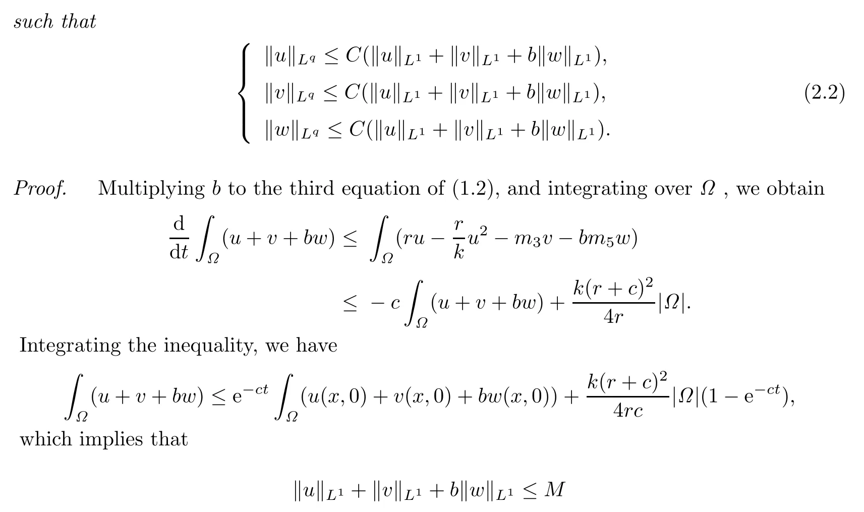
Lemma 2.1Let

For any positive solution of(1.2),there exists a positiveMsuch thatFurthermore,for eachq＞1,there exists a positive constant

for sufficiently large M.

Assuming that(2.2)holds for some q≥1(it holds for q=1 obviously from the above proof),we are to prove that it holds for exponent 2q.Multiplying the first three equations of(1.2)by u2q−1,v2q−1and w2q−1respectively,integrating overΩ,and then summing the above results,we have

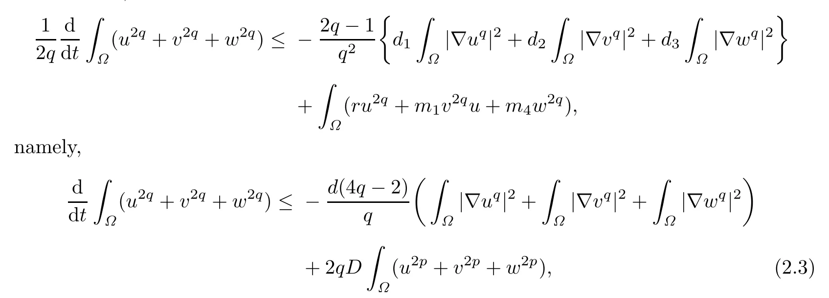
where d=min{d1,d2,d3}and D is a positive constant independent of the initial value when t is large enough.Using(2.3)and the Nirenberg-Gagliardo inequality and Young’s inequality,we see that(see[18]or[19])

for some positive constants p,where D(ǫ)is a constant depending on ǫ.Choosing

from(2.3)and(2.4),we get that there are positive constants l1and l2such that

Integrating the above inequality,the asserted estimates now follow by applying the induction hypotheses.

Theorem 2.1For any positive solution of(1.2),there exist positive constantsK1andK2such that

the first inequality in(2.6)follows by the comparison principle.

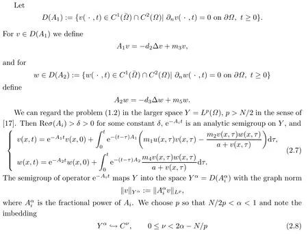
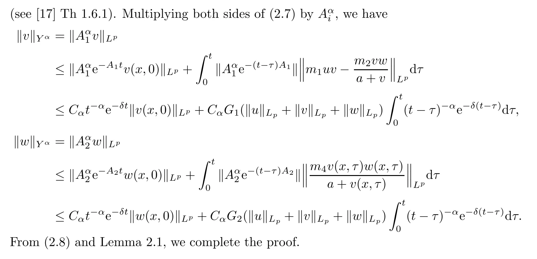
3 Stability of(u0,v0,w0):ODE system(1.1)

In this section,we consider the stability of the positive steady-state(u0,v0,w0)of(1.1). Let(u(t),v(t),w(t))be a positive solution of(1.1).It is easy to see that u(t),v(t)and w(t)are bounded(see Lemma 1 in[10]).

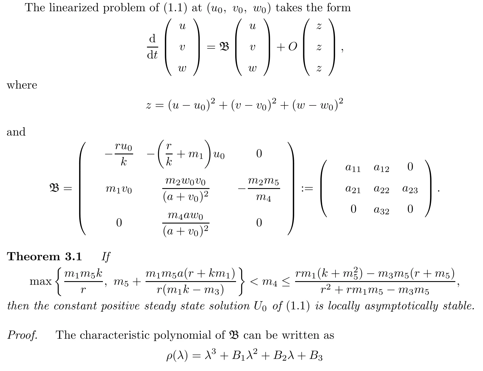
Under the conditions of the theorem,we have

Through a series of calculation,we have

We prove M＞0 under the conditions of the theorem.Notice that

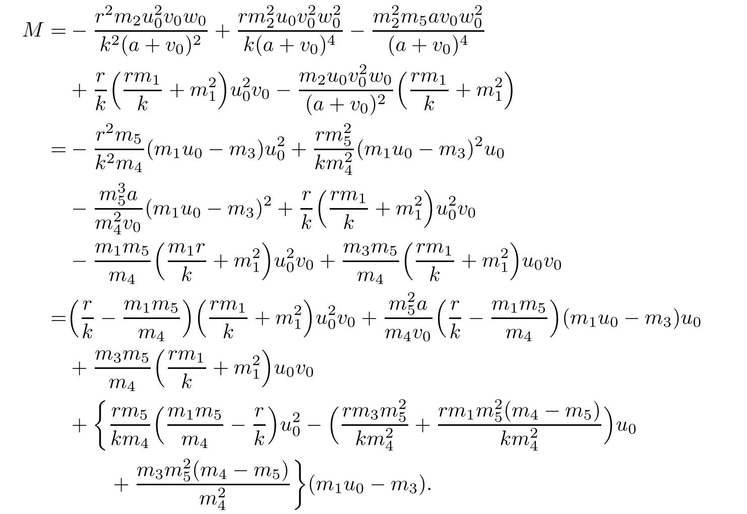
The first three terms in the right hand side of the above expression are positive if

M is positive if the expression within the curly bracket is positive.This expression can be put in the form Au2+Bu0+C,where

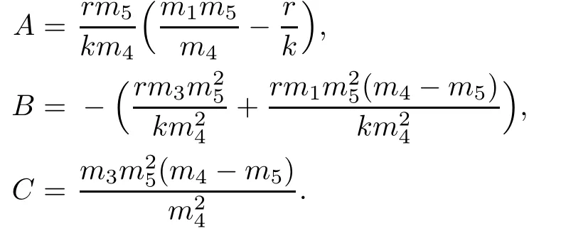
We note that A＜0,B＜0,C＞0,and thus,a sufficient condition for the positivity of this expression is Ak2+Bk+C≧0 since u0＜k,which implies

It follows from the Routh-Hurwitz criterion that the three roots λ1,λ2,λ3of ρ(λ)=0 all have negative real parts.This implies that U0is locally asymptotically stable.

4 A Priori Estimates

In this section,the main purpose is to give a priori upper bound and Harnack Inequality for positive solutions of(1.3).To this aim,we first recall the following well known results:

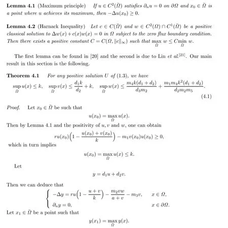
By the application of the maximum principle,it yields v(x1)≤k.Consequently,

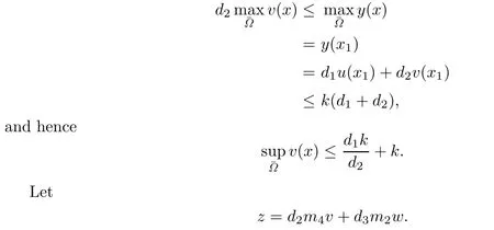
We can prove the last inequality of the theorem similarly.

Theorem 4.2Suppose that Λ is fixed.Let0＜d≤min{d1,d2,d3}be a constant.Then there exist positive constantsC1(d),C2(d,d1)andC3(d,d1)depending on Λ and Ω,such that for any positive solutionUof(1.3)the following Harnack-type inequalities holds:

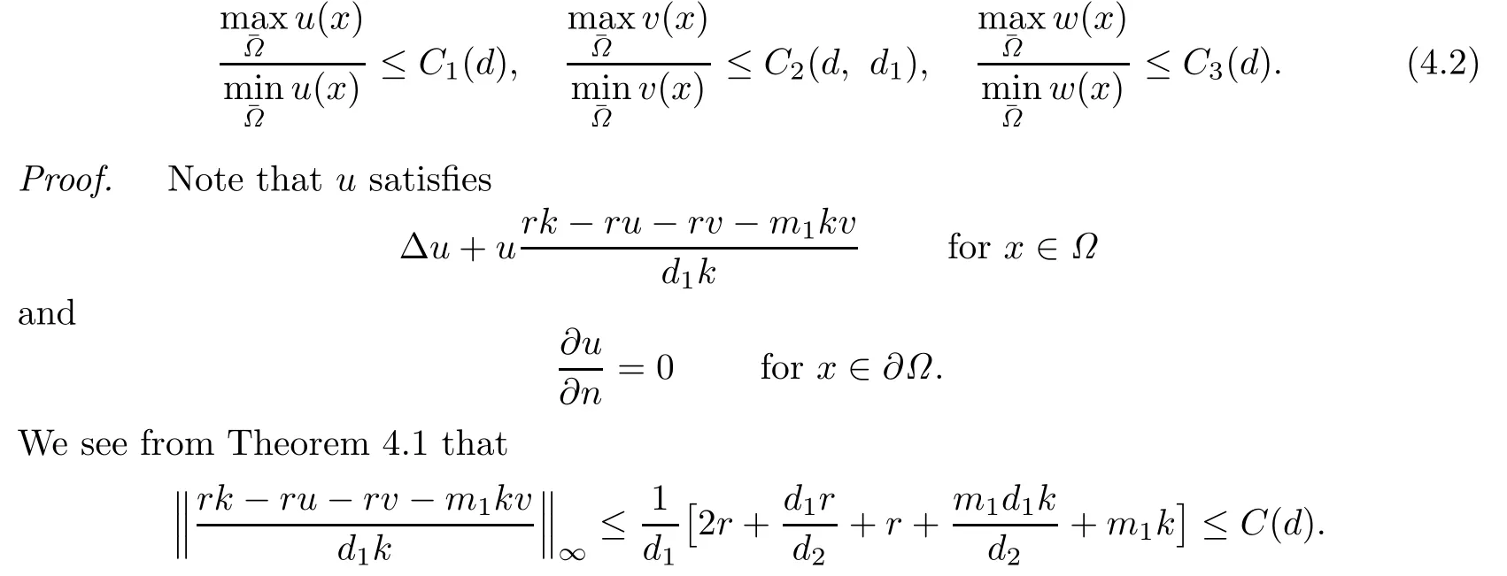
Hence it follows from Lemma 4.2 that there exists a positive constant C1(d)such that

The inequalities for v and w can be proved similarly.

5 Non-existence of Non-constant Positive Steady States

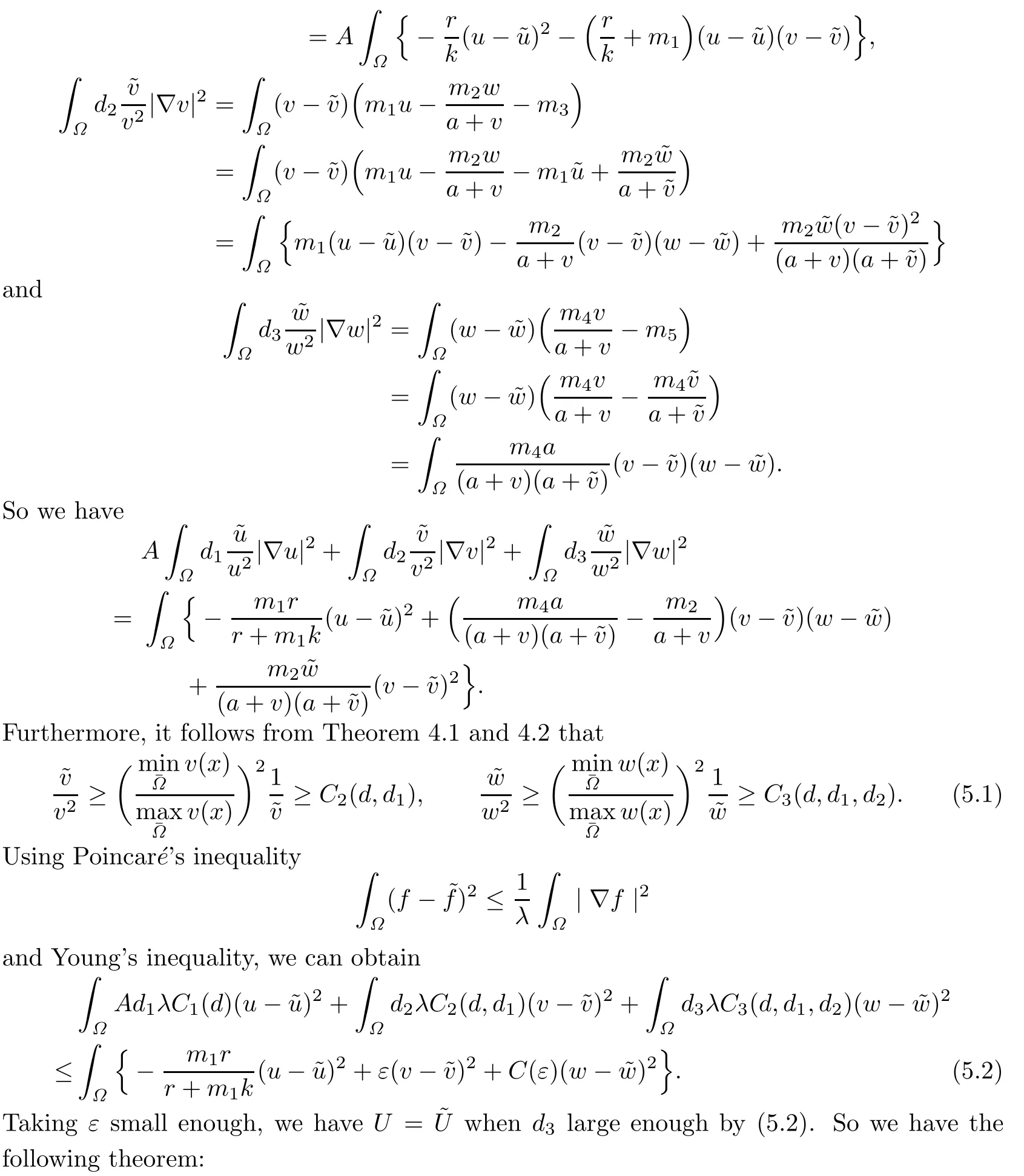
Theorem 5.1Letdbe a constant such that0＜ d≤min{d1,d2,d3}.There exist positive constantCd3=Cd3(Λ,d,d1,d2)such that the system(1.3)has no non-constant solution provided thatd3≥Cd3.

6 Bifurcation

In this section,we discuss the bifurcation of non-constant positive solutions of(1.3).Let the parametersΛ,d1,d3＞0 be fixed.And consider d2＞0 as the bifurcation parameter.

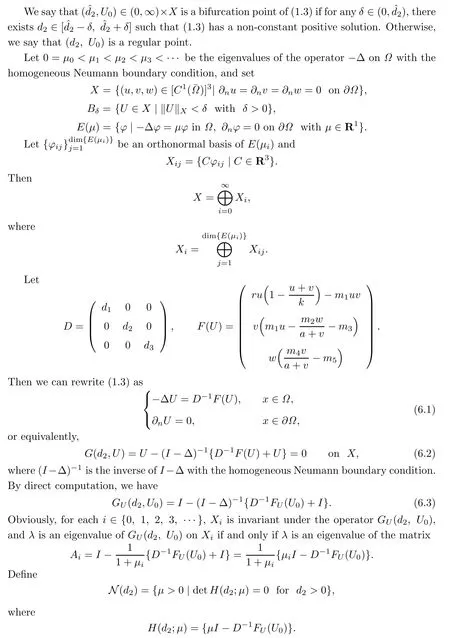
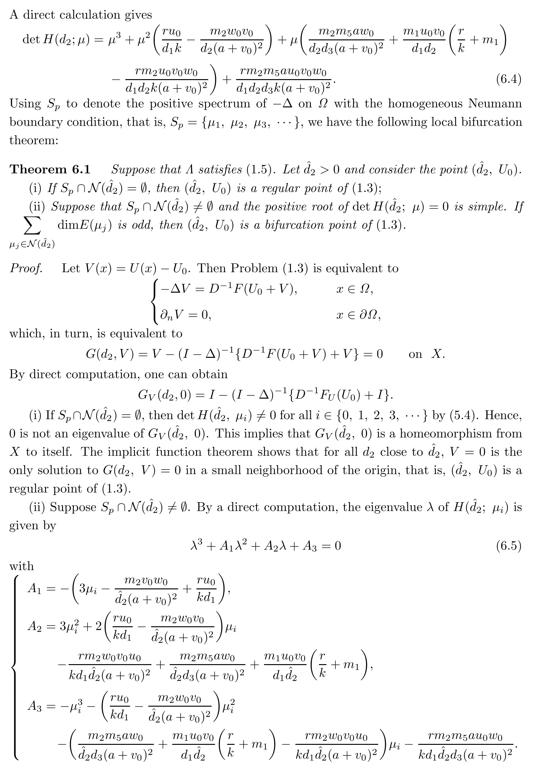
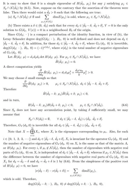
Remark 6.1From Theorems 3.1 and 6.1,we can conclude that di ff usion-driven instability occurs when the di ff usion coefficients is in a suitable range.

[1]Freedman,H.I.,A model of predator-prey dynamics modi fi ed by the action of parasite,Math. Biosci.,99(1990),143–155.

[2]Beltrami,E.and Carroll,T.O.,Modelling the role of viral disease in recurrent phytoplankton blooms,J.Math.Biol.,32(1994),857–863.

[3]Venturino,E.,Epidemics in Predator-prey Models:Disease in Prey,In:Arino,O.,Axelrod, D.,Kimmel,M.and Langlais,M.(Eds.),Mathematical Population Dynamics,Analysis of Heterogeneity,Vol.1,381–393,1995.

[4]Venturino,E.,The e ff ects of diseases on competing species,Math.Biosci.,174(2001),111–131.

[5]Venturino,E.,Epidemics in predator-prey model:disease in the predators,IMA J.Math. Appl.Med.Biol.,19(2002),185–205.

[6]Tomohito Kadota and Kousuke Kuto,Positive steady states for a prey-predator model with some nonlinear di ff usion terms,J.Math.Anal.Appl.,323(2006),1387–1401.

[7]Xiao,Y.and Chen,L.,Modelling and analysis of a predator-prey model with disease in prey,Math.Biosci.,171(2001),59–82.

[8]Chattopadhyay,J.and Pal,S.,Viral infection on phytoplankton-zooplankton system–a mathematical model,Ecological Modelling,151(2002),15–28.

[9]Hadeler,K.P.and Freedman,H.I.,Predator-prey population with parasite infection,J.Math. Biol.,27(1989),609–631.

[10]Chattopadhyay,J.and Bairagi,N.,Pelicans at risk in Salton sea-an eco-epidemiological model,Ecological Modelling,136(2001),103–112.

[11]Du,Y.H.and Lou,Y.,Qualitative behaviour of positive solutions of a predator-prey model: E ff ects of saturation,Proc.Roy.Soc.Edinburgh.,A131(2001),321–349.

[12]Pang,P.Y.H.and Wang,M.X.,Non-constant positive steady states of a predator-prey system with non-monotonic functional response and di ff usion,Proc.London Math.Soc.,88(2004), 135–157.

[13]Li,L.,Coexistence theorems of steady states for predator-prey interacting system,Trans. Amer.Math.Soc.,305(1988),143–166.

[14]Lou,Y.and Ni,W.N.,Di ff usion vs cross-di ff usion:an elliptic approach,J.differential Equations,154(1999),157–190.

[15]Pang,P.Y.H.and Wang,M.X.,Strategy and stationary pattern in a three-species predatorprey model,J.differential Equations,200(2004),245–273.

[16]Brown,P.N.,Decay to uniform states in ecological interactions,SIAM J.Appl.Math., 38(1980),22–37.

[17]Henry,D.,Geometric Theory of Semilinear Parabolic Equations,Lecture Notes in Math.,Vol. 840,Springer-Verlag,Berlin,New York,1993.

[18]Le Dung,Hal and Smith,L.,A parabolic system modelling microbial competition in an unmixed bio-reactor,J.differential Equations,130(1996),59–91.

[19]Alikakos,N.,LpBounds of Solutions of Reaction-Di ff usion Equations,Comm.Partial differential Equations,4(1979),827–868.

[20]Lou,Y.and Ni,W.M.,Di ff usion,self-di ff usion and cross-di ff usion,J.differential Equations, 131(1996),79–131.

[21]Lin,C.S.,Ni,W.M.and Takagi,I.,Large amplitude stationary solutions to a chemotaxis system,J.differential.Equations,72(1988),1–27.

35J55,37G35,92D25

A

1674-5647(2010)01-0027-14

date:May 19,2008.

The NSF(10771085)of China,the Key Lab of Symbolic Computation and Knowledge Engineering of Ministry of Education,and the 985 program of Jilin University.