Prediction of undeformed chip thickness distribution and surface roughness in ultrasonic vibration grinding of inner hole of bearings

Yanqin LI,Daohui XIANG,Guofu GAO,Feng JIAO,Bo ZHAO

School of Mechanical and Power Engineering, Henan Polytechnic University, Jiaozuo 454000, China

Abstract: Ultrasonic vibration grinding differs from traditional grinding in terms of its material removal mechanism.The randomness of grain-workpiece interaction in ultrasonic vibration grinding can produce variable chips and impact the surface roughness of workpiece.However,previous studies used iterative method to calculate the unformed chip thickness (UCT),which has low computational efficiency.In this study,a symbolic difference method is proposed to calculate the UCT.The UCT distributions are obtained to describe the stochastic interaction characteristics of ultrasonic grinding process.Meanwhile,the UCT distribution characteristics under different machining parameters are analyzed.Then,a surface roughness prediction model is established based on the UCT distribution.Finally,the correctness of the model is verified by experiments.This study provides a quick and accurate method for predicting surface roughness in longitudinal ultrasonic vibration grinding.

Key words: Ultrasonic vibration grinding;Undeformed chip thickness (UCT);Distribution characteristics;Surface roughness

1 Introduction

Ultrasonic vibration grinding is a non-traditional machining method that applies ultrasonic waves to the machining process (Chen FJ et al.,2010;Chen HF et al.,2013).Longitudinal ultrasonic vibration-assisted grinding has the advantages of improving machining quality and reducing surface roughness (Yang et al.,2020;Ding et al.,2022).In the ultrasonic vibration grinding process,grains cut the workpiece surface and produce numerous undeformed chips.The stochastic properties of grain location and protrusion height determine the undeformed chip thickness (UCT).It is useful to describe UCT quantitatively to obtain a deeper understanding of the ultrasonic vibration grinding process.

Grinding is a complex process with many random factors.Many assumptions have been applied to calculate the UCT to reduce the complexity.Hecker and Liang (2003) assumed that the UCT distribution followed a Rayleigh distribution and the surface groove profile was a triangle,and derived the workpiecesurface roughness (Ra) prediction model using UCT.Agarwal and Venkateswara Rao (2005,2010) established several analytical models of surface roughness assuming that the groove profile was semicircle or paraboloid.A new model considering the influence of overlap demonstrated higher precision (Agarwal and Venkateswara Rao,2013).Malkin and Guo (2008) proposed a maximum UCT formula and introduced the height difference between adjacent abrasive particles (δn) to consider the static height difference between adjacent grains.Subsequently,Ding et al.(2017) proposed an improved equation that considered the effect of kinematics.They studied the UCT distribution of a textured cubic boron nitride (CBN) wheel,ignoring the randomness of grains.Setti et al.(2020) believed that the UCT was closely related to the grain protrusion height and evaluated the performance of UCT during micro-grinding.He et al.(2017) compared surface roughness values with and without the overlap effect in ultrasonic grinding.The theoretical values with the overlap effect were closer to the experimental results.

Studies of surface topography were conducted mainly by numerical simulation and usually based on the kinematic analysis method (Wang et al.,2017,2020).In this method,the workpiece surface topography is predicted by solving the minimum value of the intersection trajectory.Assume that the grain height obeyed a Gaussian distribution,Zhou and Xi (2002) established a workpiece topography prediction model by searching for the intersection of motion trajectories from high to low.Gong et al.(2002) generated a grinding wheel model with the random number generated by computer and simulated with Visual C++to realize the prediction ofRa.Chen et al.(2018) proposed a workpiece topography generation algorithm considering the plowing effect in ultrasonic grinding.Zhou et al.(2018,2019) proposed a new workpiece topography model considering the Poisson effect of large load in ultrasonic vibration grinding.Zhang et al.(2020)reported the combined influence of processing and ultrasonic parameters on the surface micro structure.

Although many scholars have conducted extensive studies on establishing workpiece topography models,they have rarely referred to the calculation of UCT.Darafon et al.(2013) divided the workpiece into line segments at the same time interval to calculate the UCT.This method is extremely inefficient,and lacks analysis of the distribution characteristics of UCT.Zhang et al.(2018) proposed a Newton iterative algorithm to obtain a numerical solution of the contact timet,obtained the height value of each topological point,and then calculated the UCT to obtain the UCT distribution,but the iterative algorithm is also timeconsuming.Zhang et al.(2022) used an isometric method to solve the UCT of a single grain in the contact region of ultrasonic grinding and analyzed the effect of machining parameters.However,they focused mainly on radial and tangential ultrasonic grinding.To the best of our knowledge,no studies have considered the stochastic behavior of UCT in longitudinal ultrasonic vibration grinding.

In this paper,a symbolic difference method is introduced to obtain the contact position between the grain and the workpiece.The UCTs and interference widths are calculated during the longitudinal ultrasonic vibration grinding process.Then,the UCT distribution characteristics under different machining parameters are analyzed.The relationship between the UCT distribution mean value and surface roughness is obtained.Finally,the correctness of the prediction results is verified by ultrasonic grinding experiments.This study provides a quick and accurate method for predicting surface roughness in longitudinal ultrasonic vibration grinding.

2 Grain-workpiece interaction mechanism

2.1 Kinematic modeling

Fig.1a shows a kinematic diagram of the longitudinal ultrasonic internal grinding inner hole of bearings.The grinding wheel rotates at a speed ofnsand the workpiece rotates at a speed ofnwin the opposite direction.Rwis the radius of bearing ring andRsis the wheel radius.The motion is simplified as surface grinding in Fig.1b.In thexOwycoordinate system,the originOwis set at the highest position on the left side of the workpiece.Thex-axis is in the same direction as the feed of the wheel;they-axis is in the same direction as the workpiece’s height;thez-axis is perpendicular to thexOwyplane;bwandlware the width and length of the workpiece,respectively.The movement track equation of the gritGmnat momenttis

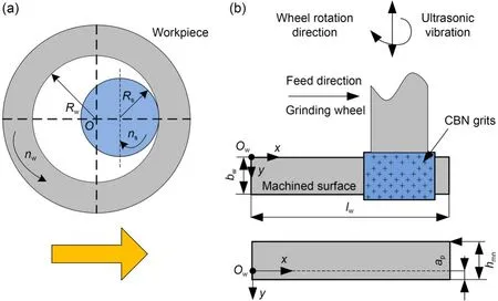
Fig.1 Establishment of the coordinate system: (a) bearing grinding diagram;(b) motion expansion diagram

where (x0,y0,z0) is the coordinate of the initial contact point between grinding wheel and workpiece;Δdand Δlare the distances between the grain and the origin in the circumferential and longitudinal directions,respectively;vwis the workpiece velocity;the index ofGmnis expressed as (m,n);hmnis the height ofGmn;hmaxis the maximum grain protrusion height;ωis the angular velocity of the grinding wheel;θis the angular displacement expressed asθ=ωt-mΔd/Rs;Ais the ultrasonic amplitude;fis the ultrasonic frequency;apis the grinding depth.The phase difference between different grinding grains is given byφ=2πfΔd/(Rsω).Because the grinding arc length is much less than the grinding wheel diameter,the simplified formulas sinθ≈θ,cosθ≈θ2/2 from Zhou et al.(2019) are used in the calculation process.Therefore,the velocity ofGmnat momenttis as follows:

2.2 Grain-workpiece interaction in the ultrasonic grinding process

The movement track of gritGmnis shown inFig.2a,and the workpiece in Fig.2b.The workpiece is discretized by Δxas a series of sampling planes in thexdirection,and the sampling plane is discretized by Δyas a series of vertical line segments.The calculation precision is determined by the sampling spacing.In Fig.2c,the length of each line segment represents the height of the workpiece.The initial value for all grid points in the height direction is set asz0.Thus,the coordinate of the grid point (xij,yij,zij) is expressed as

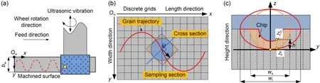
Fig.2 Chip generation mechanism illustration: (a) ultrasonic grinding diagram;(b) workpiece grids;(c) UCT and width

wherejrepresents the number of the vertical line segment within the sampling planei.

In the ultrasonic grinding contact zone,numerous grains cut the workpiece surface to achieve material removal.All cutting grains will produce chips,and the interference depths are equal to the UCTs.When the grains slide or plow across the workpiece surface,the interference depths should also be regarded as the UCTs.Therefore,the UCT can be determined by solving the interference depth.

In this study,a symbolic difference method is proposed to obtain the initial contact position of the grain and the workpiece,which significantly improves the calculation efficiency.The difference between the coordinates of the grain and the grid point is regarded as the functionf(xc) (xcis thexcoordinate of the contact position),namelyf(xc)=xc-xij.Suppose there isxcto makef(xc)=0,i.e.,xc=xij.The prerequisite for the existence of the solution of the function is thatf(xc) is a monotone function in the interval (x1,x2),andf(x1)f(x2)＜0,i.e.,f(x1) andf(x2) have different signs.Therefore,searching for the position of the contact point can be understood as the position of the function sign transformation.The steps of the symbolic difference method are as follows,and an example is shown in Table 1.

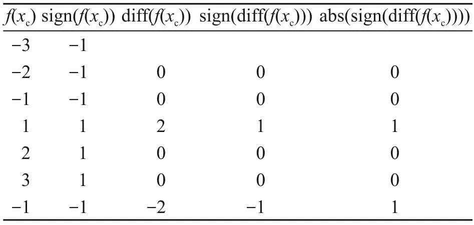
Table 1 Example of the symbolic difference method

(1) The ‘sign’ function is used to solvef(xc).Iff(xc)＜0,‘sign’ returns -1;iff(xc)＞0,‘sign’ returns 1.

(2) The difference function ‘diff’ is adopted to search the position of sign transformation.If diff(f(xc))＜0,it means the function decreases and is denoted as‘sign(diff(f(xc)))=-1’;if diff(f(xc))＞0,it means the function increases and is denoted as ‘sign(diff(f(xc)))=1’.Both cases indicate sign transformation.

(3) Searching for the contact point.Both the maximum and minimum values meet the conditions,so the‘abs’ function is used to determine the position of the contact point,i.e.,xc.

(4) The coordinate valuesycandzcare obtained according to the trajectory Eq.(1).Thus,the position of the grain can be determined.

During the longitudinal ultrasonic grinding process,the movement path of a grain on thexOwyplane is similar to a sinusoidal curve and the cross section of the grain movement path is perpendicular to the velocity direction (Fig.2b).The angleψbetween the sampling section and the cross section can be expressed as

In the sampling section,the contour of the grinding groove is an ellipse (Fig.2c).The long axis of the ellipse iswland the short axis isws.The groove contour can be expressed as

Therefore,wlis

wheredgis the diameter of the grain.

When the value ofwlis determined,the cutting groove contour Eq.(5) is determined accordingly.Fig.2c shows that the groove width generated by ultrasonic grinding is wider than that of traditional grinding.

(5) Eq.(3) is substituted into the contour Eq.(5)of grain to solvewsandwl.

Whether the grain and workpiece intersect can be determined from the interference depth and width values.Supposing that the equation is not solvable,there is no intersection between the grain and the vertical line.Instead,we can solve the equation and obtainz=zijandy=yij.This value is compared with the initial height valuez0.Ifzij＜z0,the grain intersects the vertical line (Fig.2c).Assume that the interfered workpiece material is completely removed,the interference depth ish=z0-zij,and the interference width isw=2wl.handware stored in the arraysHandW,counted asuandv,respectively.Meanwhile,considering the trajectory interference effect of grains,z0is replaced byzij.Thus,the UCT mean value in the sampling planeiis expressed as

For sampling sections at different locations,the values ofwlare different,meaning that there should be different groove contour equations,and the degree of groove widened is dynamic.Thus,the average interference width in the sampling planeiis expressed as

(6) When all sampling planes are calculated,the trajectory of a single grain cutting the workpiece surface is completed.When all grains traverse the workpiece surface according to this method,the interference depths between all grains and the workpiece can be obtained under given processing condition.When all the grains pass through the workpiece surface,the initial surface residual heightwill be updated as Eq.(9),and the machined surface height of the workpiece can be obtained.

The grain numberNon the grinding wheel surface determines the simulated workpiece surface.In the simulation process,a workpiece surface with a length of 1.5 mm was processed by 1880 grains.The flow of the surface topography and the calculation of UCT distribution algorithm are shown in Fig.3.

Fig.3 Flowchart of workpiece surface topography and UCT distribution generation algorithm

In Fig.3,nis the number of grain randomly generated;kis the calculated grain number;vsis the velocity of the grinding wheel;dg∈N(μ, σ2) representsdgfollows the normal distribution;μis the average value;σis the standard deviation;δi∈U(c,d) represents the grain position offsetδifollows the uniform distribution;canddare the upper and lower bounds,respectively.

2.3 Influence rule of machining parameters on UCT distribution

2.3.1 UCT distribution characteristics

Based on the above numerical simulation method,under the conditions of grinding parametersns=2000 r/min,vw=1200 mm/min,ap=20 μm,andA=4 μm,the grain protrusion height follows a normal distribution (Fig.4a),and the UCT distribution result is as shown in Fig.4b.The UCT distribution is represented by a probability density histogram from which the frequency variation of UCT in a specific range can be observed.The minimum cutting thickness is 0 μm,indicating that grains are not involved in the grinding.The maximum chip thickness is 13 μm.

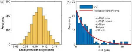
Fig.4 Numerical simulation results: (a) grain protrusion height distribution;(b) UCT distribution

An exponential function is used to fit the histogram,and its probability density function can be expressed as

and the expected valueE(h) of the exponential distribution is

whereχis the rate parameter and can be calculated by the mean value of UCT.

In addition,the mean UCT valuehmean,the maximum chip thicknesshmax,and the variancevarof the UCT distribution can all be used as quantitative characteristic parameters to describe the UCT distribution.

2.3.2 Influence rule of ultrasonic parameters on the UCT distribution

The motion trajectories of the grains in longitudinal ultrasonic grinding differ from those in traditional grinding,so the UCT distribution forms are also different.The UCT distribution histograms obtained under different ultrasonic amplitudes and frequencies shown in Fig.5 are based on the grinding parametersns=2000 r/min,vw=1200 mm/min,andap=20 μm.These UCT distributions follow an exponential distribution.The characteristic parameters extracted from the UCT distributions under different ultrasonic amplitudes and frequencies are shown in Tables 2 and 3.

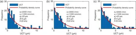
Fig.5 UCT distribution histograms under different ultrasonic amplitudes and frequencies (a-c)

As shown in Table 2,with the increase ofA,hmaxincreases from 11.8435 to 12.5179 μm;hmeandecreases from 2.5225 to 2.3802 μm;varincreases from 6.9264 to 7.2799 μm;Neincreases from 136 to 142.This is because the sinusoidal grain movement track of ultrasonic grinding is longer than the linear track of traditional grinding,causing the UCT to be more uniform and smaller.Thewmeanbetween the grain and workpiece also increases gradually,indicating that the width of the grinding groove increases.This provides the basis for obtaining a better surface than traditional grinding.It can be concluded that the ultrasonic amplitude affects the UCT distribution.

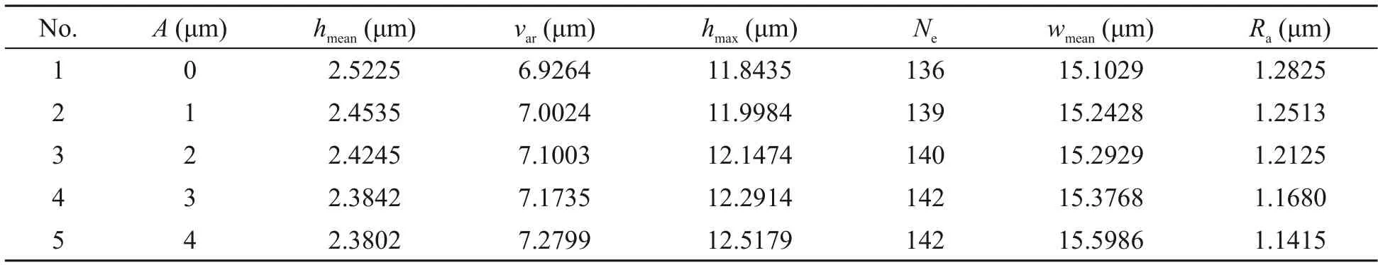
Table 2 UCT distribution parameters under different ultrasonic amplitudes

As shown in Table 3,with the increase off,the parameters such ashmaxandhmeanfirst increase and then decrease;Neremains unchanged;wmeanincreases;Rashows the same change trend ashmean.According to the above analysis,longitudinal ultrasonic grinding can improve the workpiece surface quality.Because the sine trajectory of ultrasonic grinding is superimposed,the UCT mean value decreases,and the grinding grooves are widened,and the increase ofAenhances the repeated interference effect,which is the fundamental reason for the reduction of surface roughness.

2.3.3 Influence rule of machining parameters on UCT distribution

Fig.6 shows the UCT distribution histograms at different machining parameters.For all probability density histograms,they follow the exponential distribution.

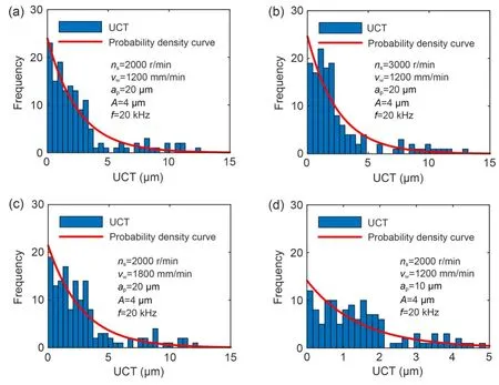
Fig.6 UCT distribution histograms under different machining parameters (a-d)

Obviously,there are significant differences in UCT distribution at different machining parameters.Whennsincreases,the number of grains with chip thickness between 0 and 5 μm increases (Figs.6a and 6b).hmaxdecreases,which means that the chip thickness distribution tends to be concentrated.hmeanandNedecrease.This is because with the increase ofns,hmaxdecreases and the radial interference depth of the grinding wheel decreases,resulting in the reduction ofNe.Meanwhile,under the samevw,whennsincreases,the workpiece feed decreases within the time interval of adjacent abrasive motion;the chip thickness of a single grain decreases;hmeandecreases;Radecreases correspondingly from 1.4172 to 0.9801 μm (Table 4).

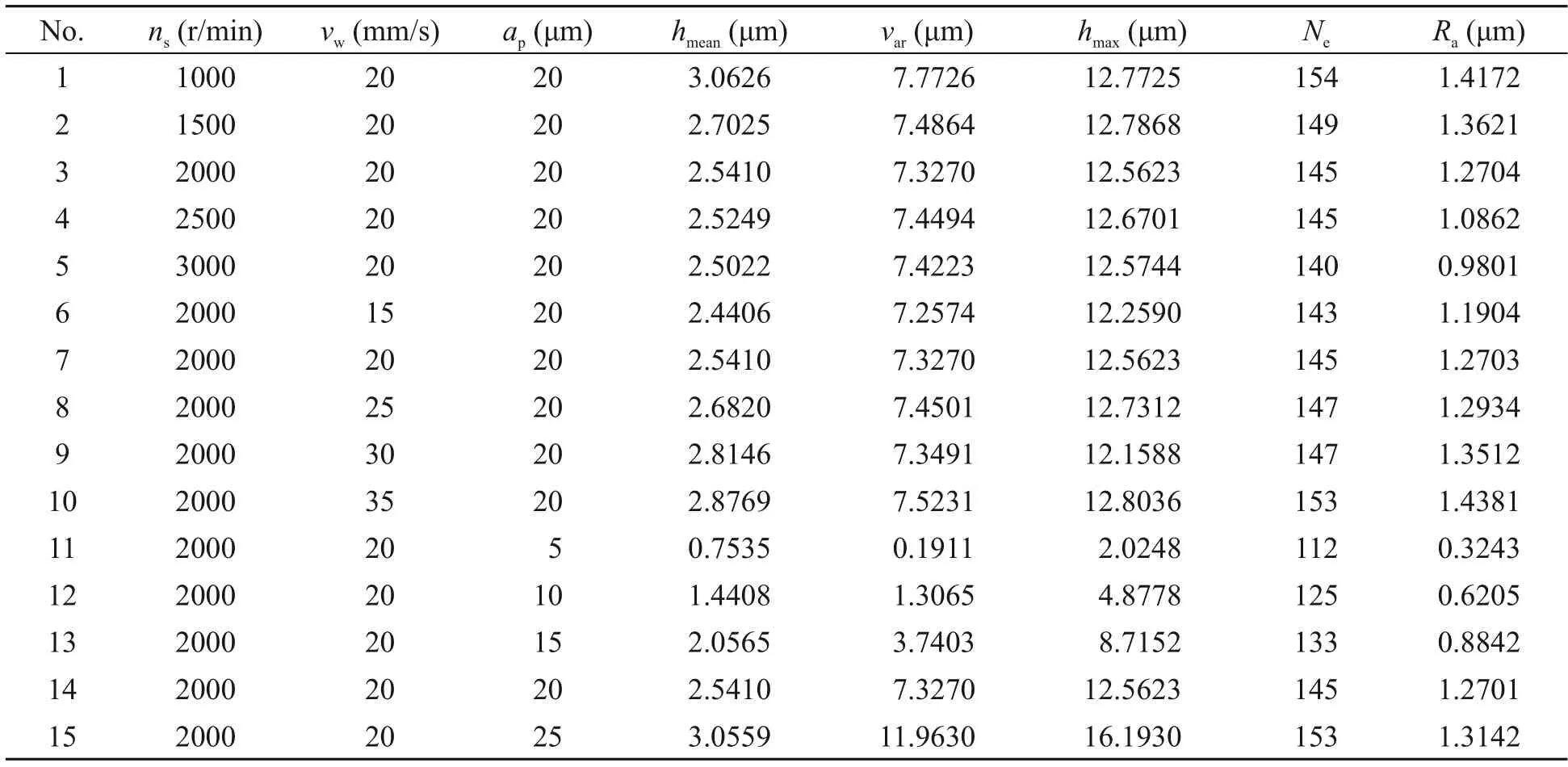
Table 4 UCT distribution parameters under different grinding parameters

The effect of thevwon the UCT distribution is shown in Figs.6a and 6c.With the increase ofvw,the number of grains with chip thickness between 0 and 5 μm decreases;hmaxincreases;hmeanincreases.varincreases,andNerises from 143 to 153.This is because asvwincreases,the radial interference depth increases,resulting in the rise ofNeandhmean,and a corresponding increase inRafrom 1.1904 to 1.4381 μm.

The effect ofapon the UCT distribution is shown in Figs.6a and 6d.With the increase ofap,hmaxincreases from 2.0248 to 16.1930 μm,indicating that the range of chip thickness distribution becomes dispersed.hmeanincreases from 0.7535 to 3.0559 μm,andvarincreases from 0.1911 to 11.9630 μm.The UCT distribution becomes more and more uneven,andRaincreases correspondingly from 0.3243 to 1.3142 μm(Table 4).

2.4 Regression model of surface roughness

The mapping relationship betweenhmeanandRacan be established from the data in Table 3,as illustrated in Eq.(12) and Fig.7.

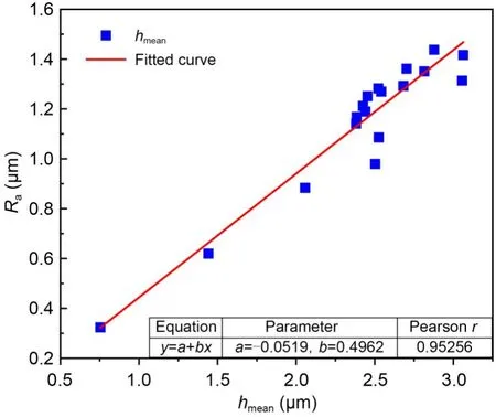
Fig.7 Relationship between hmean and Ra

whereaandbare the intercept and slope of the regression line,which are -0.0519 and 0.4962,respectively.The Pearson correlation coefficient is 0.95256.In statistics,the Pearson correlation coefficient is used to evaluate the correlation between two variables.A value between 0.8 and 1.0 is regarded as indicating a strong correlation (Tao et al.,2022).

As shown in Fig.7,Rais proportional tohmeanand the data fall on the fitted line with little deviation.This means that thehmeanreflects the stochastic characteristics of the grains and has a direct influence onRa.The establishment of the mapping relationship between thehmeanandRaprovides an effective way to predict surface roughness.

3 Experimental verification

3.1 Experimental scheme

To verify the proposed surface topography model and theRapredictive effect,a single factor experiment of ultrasonic grinding was carried out.Fig.8 shows the experimental platform,which includes ultrasonic generator,ultrasonic tool holder,and force measuring system.The ultrasonic generator generated the current signal and transmitted it to the transducer.The transducer converted received high-frequency electrical signals into mechanical signals.The horn amplified mechanical signals to produce vibration.The ultrasonic tool holder was installed on the spindle (Fig.8b).The amplitude was 4 μm and the frequency was 35 kHz.A dynamometer (Kistler 9257B,Kistler,Switzerland) was used to measure the grinding force.

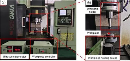
Fig.8 Diagram of the ultrasonic grinding experimental platform (a) and platform details (b)

The diameter of the ceramic bonded CBN grinding wheel was 30 mm.The workpiece was made of GCr15 bearing steel cut into rectangular blocks of 20 mm×15 mm×10 mm.The grain size was 100# and the grinding wheel concentration was 100%.The grinding wheel was dressed by a diamond roller.The dressing parameters were: speed ratioq=0.6,dressing speedvfd=300 mm/min,and dressing depthad=2 μm,and the wheel was dressed three times during every experiment.Grinding parameters are listed in Table 5.

Table 5 Grinding parameters used in the experiment

3.2 Experimental results

3.2.1 Surface topography

The surface topography of the workpiece is an intuitive index to judge the surface quality.Fig.9 shows a comparison of measured and simulated morphologies under different amplitudes (ns=2000 r/min,vw=20 mm/s,andap=20 μm).Figs.9a-9c show the workpiece surface morphologies measured by microscopy(VHX-2000C,Keyence,Japan).Figs.9d-9f show the simulated workpiece surface morphologies.

Fig.9 Surface morphology under different ultrasonic amplitudes: (a-c) measured morphology with A=0 μm (a), A=2 μm (b),and A=4 μm (c);(d-e) simulated morphology with A=0 μm (d), A=2 μm (e),and A=4 μm (f).References to color refer to the online version of this figure

The movement trajectory of grains was mapped to the workpiece surface,and surface quality was reflected through the characteristics of the grooves on the workpiece surface.As shown in Figs.9a and 9d,parallel linear grooves were formed along the grinding direction in the traditional grinding process,and an obvious plastic accumulation phenomenon occurred(Fig.9a),which affected the surface roughness of the workpiece.

The workpiece surface morphologies of ultrasonic vibration grinding underA=2 and 4 μm are shown in Figs.9b and 9c.Compared with traditional grinding,the sinusoidal trajectory of the grains forms a wavy texture on the workpiece surface.The wavy lines in Fig.9c become more curved.The range of motion trajectories of the grains is extended;the grooves are denser;the repetition rate of grinding grooves between axial and circumferential adjacent grinding grains is staggered,and a relatively flat surface topography can be obtained.The simulated workpiece surface morphologies present similar characteristics (Figs.9e and 9f).

The ultrasonic grinding process can form a wavy texture due to the grain’s sinusoidal trajectory.As the ultrasonic amplitude increases,the waves become more apparent.These results prove that the simulation model can obtain the morphological characteristics of ultrasonic grinding under different machining parameters.

3.2.2 Surface texture

The measured and simulated surface texture results at three typical wheel speeds (1000,2000,and 3000 r/min) are shown in Fig.10.

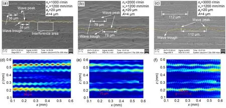
Fig.10 Surface texture under different wheel speeds: (a-c) measured texture with ns=1000 r/min (a),ns=2000 r/min (b),and ns=3000 r/min (c);(d-e) simulated texture with ns=1000 r/min (d),ns=2000 r/min (e),and ns=3000 r/min (f).References to color refer to the online version of this figure

The experimental results were affected by many factors,including grain wear and the vibration of the machine tool.Therefore,the texture morphology was not perfect.The texture spacing of the machined surface can be measured by the distance between adjacent wave troughs of the texture structure.

There were repeated wave-like textures on both the measured and simulated surfaces due to the ultrasonic vibration.The shape and distribution of the texture structure of simulation results were similar to those of the experimental results.Both results showed that the size of the texture structure was related to the wheel speed.On the measured surface,the texture spacing was nearly 38,78,and 112 μm at wheel speeds of 1000,2000,and 3000 r/min,respectively.On the simulated surface,the corresponding texture spacing was nearly 36,72,and 108 μm,respectively.The simulated spacings closely matched the measured spacings.In addition,the number of texture structures from the experimental results was the same as that from the simulation results.

The comparison between the simulation and the experimental results shows that the proposed model can describe the shape and spacing of the texture structures in ultrasonic vibration grinding,which indicates the feasibility of our proposed model.

3.2.3 Surface roughness

The surface roughness of the workpiece under different machining parameters was measured using a surface contact profiler Time 3231 (Time,China).To reflect the surface roughness fully and reasonably,after taking five measurements perpendicular to the grinding direction at different positions,the average value was calculated as the experimental results.Fig.11 shows the simulation and experimental results.

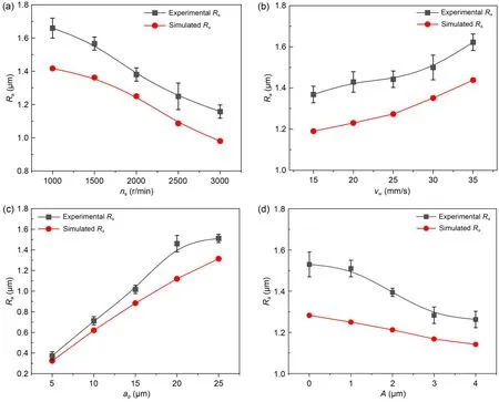
Fig.11 Surface roughness under different grinding parameters: (a) influence of wheel speed;(b) influence of workpiece velocity;(c) influence of grinding depth;(d) influence of ultrasonic amplitude

Whennsincreases,Radecreases (Fig.11a).This is because whennsincreases,the mean value of the UCT distribution decreases,the overall level of chip thickness decreases,and the distribution variance decreases.The distribution becomes more uniform.Therefore,Radecreases accordingly.

Figs.11b and 11c show thatRaincreases with the increase ofvwandap.The influence ofvwandapon the distribution characteristics of UCT is opposite to that ofns.Whenvwandapincrease,the overall level of chip thickness increases,andhmeanincreases correspondingly,which leads to the rise ofRa.

In addition,whenAincreases,Radoes not change much.It tends to decrease,which may be due to the high dressing depth,which flattens the grains and results in the insignificant ultrasonic effect (Fig.11d).In short,the variation trend of experimental results is consistent with the simulated values.The error between the simulated roughness and the experimental roughness is 14.3% at most,which verifies the model’s effectiveness.The deviation between experimental and simulation results is due to the effect of uncontrollable factors such as grain wear and spindle vibration.

4 Conclusions

This study provides a quick and effective method to calculate UCT and width in longitudinal ultrasonic vibration grinding,and a surface roughness prediction model related to the UCT distribution characteristics.The following conclusions can be summarized:

1.Based on the grain moving trajectory during ultrasonic vibration grinding,a symbolic difference method was proposed to calculate UCT and width to raise the simulation efficiency.

2.The UCT distribution in the ultrasonic vibration grinding process follows an exponential distribution.The characteristic parameters of UCT distribution were extracted.The application of ultrasonic waves can change UCT and width,enhance the repeated interference effect,and reduce the surface roughness.

3.The influence rules of grinding parameters on the UCT distribution characteristics were analyzed.A linear relationship is found betweenRaandhmean.The experimental results show the same variation tendency as the simulated values,with a maximum deviation of 14.3%.

4.High grinding wheel speed,low workpiece speed,small grinding depth,and an appropriate ultrasonic amplitude are conducive to obtaining lower UCT,forming a smoother workpiece surface.

Acknowledgments

This work is supported by the National Key Research and Development Program of China (No.2018YFB2000402),the Open Fund Project of Xinchang Research Institute of Zhejiang University of Technology,and the Fundamental Research Funds for the Universities of Henan Province,China(No.NSFRF200102).

Author contributions

Yanqin LI investigated and wrote the original draft.Daohui XIANG processed the corresponding data.Guofu GAO helped organize the manuscript.Feng JIAO helped modify the manuscript.Bo ZHAO designed the research.

Conflict of interest

Yanqin LI,Daohui XIANG,Guofu GAO,Feng JIAO,and Bo ZHAO declare that they have no conflict of interest.