Attribution of Biases of Interhemispheric Temperature Contrast in CMIP6 Models

Shiyan ZHANG,Yongyun HU*,Jiankai ZHANG,and Yan XIA

1Laboratory for Climate and Ocean-Atmosphere Studies, Department of Atmospheric and Oceanic Sciences,School of Physics, Peking University, Beijing 100871, China

2College of Atmospheric Sciences, Lanzhou University, Lanzhou 730000, China

3School of Systems Science, Beijing Normal University, Beijing 100875, China

ABSTRACT One of the basic characteristics of Earth’s modern climate is that the Northern Hemisphere (NH) is climatologically warmer than the Southern Hemisphere (SH).Here,model performances of this basic state are examined using simulation results from 26 CMIP6 models.Results show that the CMIP6 models underestimate the contrast in interhemispheric surface temperatures on average (0.8 K for CMIP6 mean versus 1.4 K for reanalysis data mean),and that there is a large intermodel spread,ranging from -0.7 K to 2.3 K.A box model energy budget analysis shows that the contrast in interhemispheric shortwave absorption at the top of the atmosphere,the contrast in interhemispheric greenhouse trapping,and the crossequatorial northward ocean heat transport,are all underestimated in the multimodel mean.By examining the intermodel spread,we find intermodel biases can be tracked back to biases in midlatitude shortwave cloud forcing in AGCMs.Models with a weaker interhemispheric temperature contrast underestimate the shortwave cloud reflection in the SH but overestimate the shortwave cloud reflection in the NH,which are respectively due to underestimation of the cloud fraction over the SH extratropical ocean and overestimation of the cloud liquid water content over the NH extratropical continents.Models that underestimate the interhemispheric temperature contrast exhibit larger double ITCZ biases,characterized by excessive precipitation in the SH tropics.Although this intermodel spread does not account for the multimodel ensemble mean biases,it highlights that improving cloud simulation in AGCMs is essential for simulating the climate realistically in coupled models.

Key words: interhemispheric temperature contrast,energy balance,shortwave cloud forcing,ITCZ,CMIP6,AGCM

1.Introduction

Interhemispheric temperature contrast is of great importance for the climatology of,and changes in,tropical atmospheric circulations and precipitation.It strongly affects the tropical monsoon systems from seasonal to multidecadal scales (Chiang et al.,2008;Ayliffe et al.,2013;Talento and Barreiro,2018).Modeling studies suggest that the latitude of the intertropical convergence zone (ITCZ) and the ascending branch of the Hadley circulation tend to shift meridionally to the anomalously warmer hemisphere (Chiang and Friedman,2012;Schneider et al.,2014).Similar linkages also exist in paleoclimates (Toggweiler and Lea,2010;Han et al.,2023) when the interhemispheric thermal contrast changed a lot due to changes in Earth’s orbit,CO2concentration,vegetation,and ice sheets (Neukom et al.,2014).In the presentday climate,the Northern Hemisphere (NH) is warmer than the Southern Hemisphere (SH) in terms of the annual mean state.It has been shown that such an interhemispheric temperature contrast will enhance significantly in response to increasing greenhouse gas concentrations in the future (Friedman et al.,2013).Thus,accurate simulation of the contrast in interhemispheric temperatures is very important for studying climate changes in the past,present,and future.

In spite of robust increasing trends in interhemispheric temperature contrast projected by climate models,significant biases remain in the climate mean state,and these biases can be traced to model deficiencies in simulating atmospheric processes and ocean circulations,as well as atmosphereocean coupling and feedback.For example,Meijers (2014)reported that CMIP5 models have warm SST biases over the Southern Ocean and that these biases are closely linked to excessive downward shortwave radiation at the surface due to cloud errors (Trenberth and Fasullo,2010;Hu et al.,2011;Hyder et al.,2018).Wang et al.(2014) suggested that the warm SST bias in the Southern Ocean and cold SST bias in the NH in CMIP5 models can be attributed to the simulated weak Atlantic Meridional Overturning Circulation(AMOC).A weak AMOC is associated with reduced northward ocean heat transport (OHT),which leads to cooling of the North Atlantic Ocean and warming of the Southern Ocean.The associated North Atlantic SST biases further lead to cold North Pacific SST anomalies through atmospheric teleconnections and air-sea feedback (Zhang and Delworth,2007).In addition to SST biases,CMIP5 models also exhibit substantial intermodel spread in temperatures over land (Zhou and Xie,2017),which is possibly due to significant differences in surface albedo related to the simulated snow cover (Wang et al.,2016) and vegetation cover(Brovkin et al.,2013).In general,the above-mentioned processes all affect the performance of models in simulating the interhemispheric temperature contrast,yet their relative importance in causing these deviations has not been quantified.

Using an energy balance box model,Kang et al.(2015)quantified the causes of the interhemispheric temperature difference in Earth’s modern climate.It was found that the northward cross-equatorial OHT is essential to maintain the warmer NH and colder SH.This interhemispheric temperature contrast caused by OHT is further enhanced by positive water vapor-greenhouse feedback,which leads to greater greenhouse trapping in the NH than the SH.The positive contributions from these two processes are then partly compensated for by the southward meridional atmospheric energy transport by the thermally driven atmospheric circulation.The interhemispheric contrast in shortwave absorption caused by the interhemispheric difference in planetary albedo plays only a minor role.This box model allows us to quantify the performance of CMIP6 models in simulating the above processes.

In this study,we evaluate the biases of interhemispheric surface temperature contrast in 26 CMIP6 models and quantify the contributions from different processes.It turns out that CMIP6 models underestimate the interhemispheric surface temperature contrast on average.The interhemispheric contrast in shortwave radiation at the top of the atmosphere(TOA),the interhemispheric contrast in greenhouse trapping,and the cross-equatorial northward OHT,are all underestimated.Also,the interhemispheric surface temperature contrast exhibits large intermodel spread,likely caused by cloud biases in AGCMs.

The rest of this paper is organized as follows.The data and methods are described in section 2,followed in section 3 by an assessment of the performances of CMIP6 models in simulating the climatological interhemispheric temperature contrast,an attribution analysis of the intermodel spread,and an examination of the possible future changes.Conclusions and some further discussion are provided in section 4.

2.Data and methods

2.1.Data

We focus on the climatological mean state from 1979 to 2014.Two experiments from each of 26 models participating in CMIP6 are analyzed,including the fully coupled historical simulation and the AMIP simulation forced with prescribed SST.The global surface temperature,radiation,and cloud outputs are investigated.All data are interpolated into a horizonal 2°×2° grid.The results of future projection during 2015-2100 are also analyzed,based on outputs of the SSP5-8.5 scenario.Details of the models are given in Table 1.

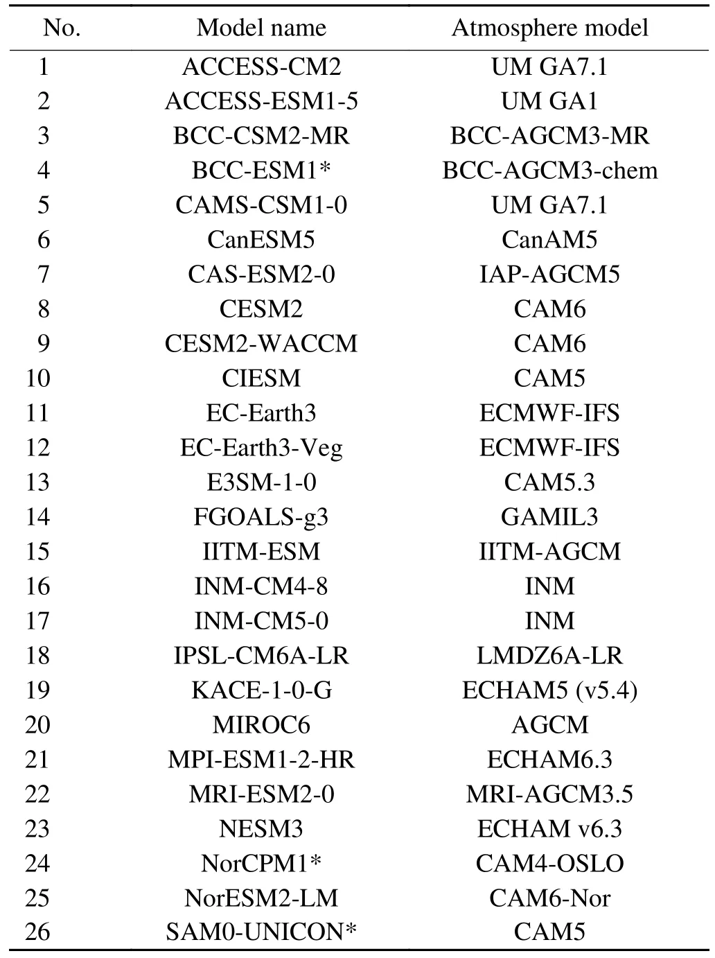
Table 1.Details of the 26 CMIP6 models used in this study.All models have available outputs of Historical/AMIP simulations.Asterisks denote models with no available SSP5-8.5 simulation output.The models are numbered alphabetically,and these numbers are used in scatter plots below.

We also use two reanalysis datasets-the Kalnay et al.(1996) NCEP-NCAR reanalysis (hereafter referred to by its alternative name,Reanalysis-1) and the fifth major global reanalysis produced by ECMWF (ERA5;Hersbach et al.,2020)-from 1979 to 2014,to evaluate the models’ biases.Reanalysis-1 has a horizontal resolution of 2.5°×2.5°.ERA5 has a horizontal resolution of 1°×1°,and it uses an upgraded radiation scheme (Morcrette et al.,2008) which offers considerable improvements compared with the older version.

2.2.Methods

2.2.1.Box model

A box model based on the energy budget of each hemisphere (Kang et al.,2015) is used to solve the interhemispheric surface temperature contrast.The energy balance equations for the two hemispheres are

in which the subscripts 1 and 2 denote the NH and SH means,respectively;SW is the net incoming shortwave radiationattheTOA;σ-Grepresentsthe outgoing longwave radiation(OLR) attheTOA,whereσrepresents thesurface longwave emission,σ=5.67×10-8Wm-2K-1is the Stefan-Boltzmann constant,andG(=OLR-σ) measures the greenhouse trapping of the atmosphere;OHT and AHT are the cross-equatorial northward ocean and atmospheric heat transports,respectively,for which positive values represent northward heat transport and negative values southward heat transport;andAis the area of the hemisphere.

It follows that

The interhemispheric surface temperature difference can then be divided into four components as follows:

in which the subscript 0 denotes the global mean.Equations(5) to (8) measure the interhemispheric surface temperature difference caused by the interhemispheric SW difference,interhemisphericGdifference,cross-equatorial OHT,and cross-equatorial AHT.

The meridional ocean and atmosphere heat transport are calculated as (He et al.,2019)

where Fs=SWs-LWs-SH-LH is the net surface heat flux and Ft=SWt-LWtis the net incoming radiation at the TOA,in which SW,LW,SH,and LH represent the net shortwave radiation,net longwave radiation,surface sensible heating,and latent heating flux,respectively;φNand φSare the north and south pole,respectively;and λEand λWare the eastern and western boundary of the ocean basin,respectively.The OHT derived from the net surface heat flux includes the ocean heat content-induced heat transport and advective heat transport by ocean circulation.By comparing the OHT here with that in the pre-industrial control simulations under a fixed CO2concentration (figure not shown),it is found that the slow increase in GHGs leads to insignificant changes in the total OHT if we consider the climate mean state.

2.2.2.Planetary albedo

The planetary albedo contains the contributions from atmospheric reflection and absorption (e.g.,clouds and aerosols) as well as surface reflection (e.g.,ocean and continents),and is partitioned into the contribution from the atmosphere and surface according to Donohoe and Battisti (2011)as follows:

and

whereR,A,and α are the cloud reflection,atmospheric absorption,and surface albedo,respectively.They are estimated according to

in which the upward and downward arrows indicate the upward and downward SW radiation at the surface (subscript“surf”) or TOA,respectively.

3.Results

3.1.Climatology

Figure 1 shows the interhemispheric surface temperature contrast in all 26 CMIP6 models,which is calculated as the difference between the area-weighted mean surface temperature in the NH and SH.It is shown that the models exhibit substantial spread in simulating the warmer NH and colder SH.On average,the CMIP6 models underestimate the interhemispheric surface temperature contrast compared to the reanalysis datasets (0.8 K for the multimodel mean versus 1.3 K in Reanlysis-1 and 1.5 K in ERA5).Of the 26 models,2 (IPSL-CM6A-LR and MPI-ESM1-2-HR) capture well the interhemispheric surface temperature contrast,with their confidence intervals falling within those of the two reanalysis datasets.Twenty models underestimate the interhemispheric temperature contrast,four of which even simulate a climatologically warmer SH relative to the NH;whereas,four models overestimate the interhemispheric temperature contrast.It is worth noting that the multimodel mean intermodel surface temperature difference is～0.8 K in CMIP5 simulations (figure not shown),indicating that on average there is no significant improvement in simulating the interhemispheric surface temperature contrast from CMIP5 to CMIP6.

Figure 2a shows the latitudinal distribution of the interhemispheric surface temperature difference.The NH is warmer than the SH at low and high latitudes,while it is colder than the SH at midlatitudes.This distribution is closely related to the land-sea configuration;that is,a larger surface albedo due to the larger continental area in the midlatitude NH tends to have lower surface temperature than its SH counterpart (Fig.2b).Compared to the reanalysis datasets,the multimodel mean interhemispheric temperature difference has the largest negative bias around 60°,where the largest intermodel spread is also apparent.This underestimation of the interhemispheric temperature difference is mainly due to that over the midlatitude ocean (Fig.2c).

Fig.1.The annual mean interhemispheric surface temperature contrast in 26 CMIP6 models.Error bars show the ±1.96σ range (the 95% confidence intervals of the t-distribution) of the 36 years of data in each model.In the right part of the plot,the black cross indicates the multimodel ensemble mean,the rectangle shows the minimum and maximum values across all models,and the error bars show the confidence range across all models.Red and blue crosses indicate the results of Reanalysis-1 and ERA5,respectively.Red and blue error bars show the confidence intervals of each reanalysis dataset.The light red area indicates the confidence intervals of the two reanalysis datasets.

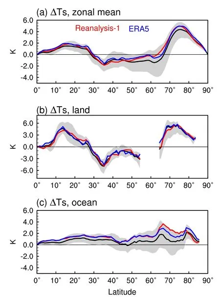
Fig.2.The latitudinal distribution of the interhemispheric surface temperature difference (weighted by cosine of latitude)for the (a) zonal mean,(b) ocean mean,and (c) land mean.Gray shading marks the intermodel spread.Red and blue lines indicate the results of Reanalysis-1 and ERA5,respectively.

We focus on the energy balance to understand the interhemispheric temperature contrast bias in CMIP6 models.Under the energy balance assumption,the net radiation at the TOA results from SW radiation absorption and longwave emission,and is redistributed between the two hemispheres by the ocean and atmospheric circulation [Eqs.(1) and (2)].The OLR at the TOA is related to the surface longwave emission and atmosphere greenhouse trapping,in which the former depends on surface temperature and the latter is a combined effect of atmospheric water vapor,cloud,and many other processes.Therefore,the contribution of the above-mentioned four components to the interhemispheric temperature contrast can be estimated quantitatively based on Eqs.(5) to(8).Figure 3a shows that these four components reproduce the interhemispheric temperature contrast well,and the residual term can be ignored (Fig.3f).The partitioning of the interhemispheric temperature contrast to these four components is a little artificial,as there are complicated interactions between different processes.Nevertheless,this method provides a concise framework for interpreting the interhemispheric temperature contrast,which is the basis for a deeper understanding.

Fig.3.The interhemispheric surface temperature contrast and contributions from different components: (a) the interhemispheric temperature contrast (white bars) and that estimated by the box model (orange bars);(b-e) contributions due to the interhemispheric difference of TOA SW (b),greenhouse trapping G (c),cross-equatorial OHT (d),and crossequatorial AHT (e).(f) The residual term that cannot be explained by the box model.The black cross indicates the multimodel ensemble mean,and error bars show the minimum and maximum values among all models.Red and blue crosses indicate the results of Reanalysis-1 and ERA5,respectively.

Fig.4.Composite differences in SW between Min3 and Max3 models (former minus latter): (a) net SW income at the TOA;(b) total reflected SW at the TOA;(c) atmospheric reflected SW at the TOA;and (c) surface reflected SW at the TOA.

The results derived from the two reanalysis datasets are firstly examined (red and blue crosses in Fig.3).It shows that both the interhemispheric greenhouse trapping contrast(G) and the cross-equatorial northward OHT lead to a warmer NH and colder SH.The cross-equatorial southward AHT acts to reduce the interhemispheric temperature contrast.These results are consistent with Kang et al.(2015).The fact that the NH has a greaterGis related to its larger land cover,and theGis greater over the continent than over the ocean (Kang et al.,2015).The climatological northward OHT is accomplished by the AMOC (Forget and Ferreira,2019),because it transports warm water into the NH in its shallow branch and returns cold water into the SH in its deep branch.The climatological southward AHT is accomplished by the Hadley circulation;its cross-equatorial southward dry static energy transport by the upper branch outweighs the northward latent heat transport by the lower branch (Kang et al.,2018).The interhemispheric temperature contrast due to net SW income at the TOA shows uncertainty between the two reanalysis datasets.The possible reason is the uncertainty in SW parameterization in the reanalysis global data assimilation system (Yang et al.,1999).For the reanalyses mean,the SW radiation plays a minor role in causing the climate-mean interhemispheric temperature contrast compared to the other three components.Over the past decade,a near symmetry of the reflected SW radiation at the TOA between the two hemispheres on the annual mean time scale has been found from various satellite datasets(Voigt et al.,2013;Stephens et al.,2015).However,the robustness of this feature and the maintaining mechanisms have been less clear to date (Stephens et al.,2016;Datseris and Stevens,2021).Some explanations include the SW cloud forcing (SWCF) of the extratropical storm track and the tropical ITCZ (Voigt et al.,2014;Bender et al.,2017),which compensate for the albedo asymmetry caused by the continents.

For the CMIP6 multimodel mean (black crosses in Fig.3),the interhemispheric temperature contrast caused by SW,Gand OHT are all underestimated compared to that in the reanalysis datasets.The resulting weaker interhemispheric surface temperature contrast is partly offset by a stronger cross-equatorial northward AHT bias.In quantitative terms,compared with the reanalysis datasets,the CMIP6 multimodel mean underestimates the interhemispheric temperature contrast by about -0.6 K,in which the contributions from SW,G,OHT,and AHT biases are -0.6 K,-0.8 K,-0.4 K,and 1.2 K,respectively.It is worth noting that although SW does not cause a large interhemispheric temperature contrast in the climate mean state,it becomes particularly important in terms of the model bias relative to the reanalysis datasets.

For individual models,the interhemispheric temperature contrast due to SW,G,and AHT show large uncertainties in their signs.Considering the three models with the largest negative interhemispheric thermal contrast biases (CAMSCSM1-0,IITM-ESM,and EC-Earth3;hereafter referred to as Min3),they exhibit negative interhemispheric temperature contrast (-0.48 K on average),since the negative contributions of the interhemispheric SW andGcontrast (-0.89 K and -0.62 K,respectively) exceed the positive contribution of OHT (1.26 K).Compared to the reanalyses mean,the Min3 mean underestimates the interhemispheric temperature contrast by about -1.9 K,in which the contributions from SW,G,OHT,and AHT biases are -1.2 K,-1.8 K,-0.3 K,and 1.3 K,respectively.These results highlight the importance of the interhemispheric contrast in SW andGin causing the Min3 bias.

The interhemispheric temperature contrast is significantly positively correlated with the contributions from SW[correlation coefficient (r)=0.71] andG(r=0.95),while negatively correlated with OHT (r=-0.44) and AHT (r=-0.50) among all models.This indicates that models with larger negative interhemispheric temperature contrast biases exhibit larger negative biases in their interhemispheric contrast in SW andG,and their biases are partially offset by positive OHT bias and AHT bias.It is worth noting that,although the northward cross-equatorial OHT is consistently represented in CMIP6 models,it is negatively correlated with the interhemispheric temperature contrast.This is likely related to the OHT response to SW bias,since the latter originates from the cloud biases in atmospheric circulation models,as will be shown in the following analyses.Changes in SW at the TOA may influence OHT by increasing oceanic stratification (He et al.,2019) and changing the ocean circulation through modulating the surface heat flux(Gregory et al.,2005) and midlatitude jet (Ceppi et al.,2013).Figures 3b and d show a significant inverse relationship between the interhemispheric SW contrast and OHT,withr=-0.72,indicating that a stronger interhemispheric SW contrast is associated with a weaker OHT in these models.

In the following analysis,we investigate the details of the intermodel spread for SW,G,OHT,and AHT,based on differences between the three Min3 models and the three models that have the largest positive interhemispheric thermal contrast bias (CESM2,CESM2-WACCM,and MRI-ESM2-0;hereafter referred to as Max3).Since the Min3 models make the largest contributions to the underestimation of the interhemispheric temperature contrast for the CMIP6 mean,the results of the Min3 models minus the Max3 models directly exhibit the possible causes of the warmer SH and colder NH biases in the Min3 models;plus,it is also helpful in understanding the CMIP6 mean biases.

Figure 4a shows the composite net SW differences between the Min3 and Max3 models.It shows positive SW biases over the midlatitude Southern Ocean (30°-60°S) and negative SW biases in the NH,especially over midlatitude East Asia and western North America.Further analysis shows that these net SW income biases are mainly from the planetary SW reflection biases rather than the TOA downward SW (Fig.3b).The Min3 models underestimate the SH planetary SW reflection but overestimate the NH planetary SW reflection.The total planetary SW reflection at the TOA is then partitioned into the contributions from atmospheric and surface reflection in Figs.4c and d,respectively.The atmospheric SW reflection is due to clouds and aerosols,and the surface SW reflection is related to snow and ice.The results show that atmospheric reflection dominates the intermodel differences of net SW at the TOA (their pattern correlation coefficient is -0.96).The intermodel differences in surface SW reflection are negligible,except over the Antarctic continent.

Figure 5a evaluates the composite differences in SWCF between the Min3 and Max3 models.The SWCF is calculated as the clear-sky SW flux at the TOA minus the all-sky SW flux at the TOA,for which a negative value represents a greater cloud SW reflection and cooling effect,while a positive value represents a lesser cloud SW reflection and warming effect.Figure 5a shows similar features as Figs.4a and b.Specifically,it shows positive SWCF anomalies over the SH midlatitude ocean and negative SWCF anomalies over the NH midlatitude continents.By constructing an interhemispheric midlatitude SWCF difference index,we show that it is significantly positively correlated with the interhemispheric temperature contrast among all 26 models (Fig.5d,black dots).These results confirm the close linkage between the midlatitude SWCF bias and the interhemispheric temperature contrast bias among the 26 models.

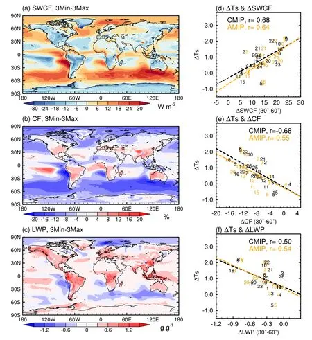
Fig.5.Relations between interhemispheric temperature contrast and cloud properties: (a-c) composite differences between Min3 and Max3 models for (a) SWCF,(b) total-area CF,and (c) cloud LWP;(d-f) scatter plots of interhemispheric temperature contrast in coupled historical simulations versus the interhemispheric difference in midlatitude (30°-60° mean) (d) SWCF,(e) CF,and (f) LWP,in coupled historical (CMIP,black) and AMIP (orange)simulations.

The SWCF biases may come from the AGCMs and be modulated by the SST biases as well as the atmosphereocean coupling processes.Next,by examining the results of AMIP simulations,we find that biases in cloud properties in AGCMs are important sources of the SWCF biases and therefore the interhemispheric temperature contrast biases.Figure 5d compares the interhemispheric midlatitude SWCF differences in AMIP simulations (orange dots) and those in coupled simulations (black dots).Although they differ slightly from each other,they both correlate well with the interhemispheric temperature contrast simulated by coupled simulations.This indicates that the interhemispheric temperature contrast in coupled models depends on the intermodel SWCF spread in AGCMs,in spite of the influence of the atmosphere-ocean coupling processes.

The SWCF biases are closely related to various cloud properties,including the cloud fraction (CF),cloud liquid/ice water content,and cloud vertical structure,which are subgrid-scale properties and estimated by cloud parameterizations in AGCMs.For a further step,we analyzed the possible linkage between the SWCF bias and cloud properties.The results suggest that the intermodel differences in total CF(Fig.5b) and cloud liquid water path (Fig.5c,LWP) are two essential factors that influence the intermodel SWCF bias and therefore the surface temperature bias.On the one hand,the Min3 models underestimate the global CF,especially over the SH midlatitude ocean,which dominates the positive SWCF biases here (their spatial correlation coefficient is 0.78).On the other hand,the Min3 models overestimate the cloud liquid water content over most continents,which intensifies cloud radiative cooling and leads to negative SWCF biases,especially over the NH midlatitude continents.These relations between SWCF and CF/LWP are consistent with Kristiansen and Kristjánsson (1999).

Figures 5e and f compare the interhemispheric differences in midlatitude CF and LWP in AMIP simulations(orange dots) and coupled historical simulations (black dots)with the interhemispheric temperature contrast in coupled historical simulations.Their significant correlations confirm that the cloud property biases in AGCMs are an important source of uncertainty in interhemispheric temperature contrast in coupled models.

The effect of cloud longwave radiative heating is evaluated in Fig.6.First,Fig.6a shows the composite difference in greenhouse trapping (G) between Min3 and Max3 models.There are positiveGanomalies in the whole SH,especially for the SH tropical eastern Pacific/Atlantic Ocean stratocumulus cloud region and the Southern Ocean.There are negativeGanomalies in most regions of the NH,mainly over the Atlantic Ocean and continental Africa.Figures 6b and c show that this intermodel spread in the interhemisphericGcontrast derives mainly from the clear-sky greenhouse trapping,i.e.,the infrared absorption of greenhouse gases,rather than the cloud longwave radiative heating.The longwave cloud forcing only has some weak contributions over the SH marine stratocumulus cloud regions.

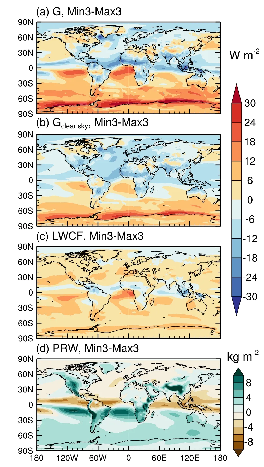
Fig.6.Composite differences in longwave trapping and column-integrated water vapor between the Min3 and Max3 models (former minus latter): (a) greenhouse trapping;(b)clear-sky greenhouse trapping;(c) longwave cloud forcing;and (d) column-integrated water vapor content.

Figure 6 d shows the composite differences in columnintegrated water vapor content (also known as precipitable water) between Min3 and Max3 models.It shows that the Min3 models have more water vapor in the warmer SH,which prevents longwave radiation loss and leads to stronger greenhouse trapping in the SH.

Figures 7a and b show the latitudinal profiles of the meridional oceanic and atmospheric heat transport in Min3 and Max3 models.Both OHT and AHT are expected to produce a larger interhemispheric temperature contrast in the Min3 models.The cross-equatorial northward OHT is stronger in the Min3 than Max3 models.The magnitude of the cross-equatorial AHT is relatively weaker,but differs in sign,in Min3 compared with Max3 models: Min3 models have northward cross-equatorial AHT,which tends to increase the interhemispheric temperature contrast.Meanwhile,the Min3 models exhibit warmer SH and colder NH biases,indicating that the negative interhemispheric temperature contrast bias caused by SW andGoverwhelm the positive bias caused by the cross-equatorial northward OHT and AHT in Min3 models.Figures 7d and e show significant negative cross-model correlations between the interhemispheric temperature contrast and cross-equatorial OHT (Fig.7d,r=-0.43) and AHT (Fig.7e,r=-0.49),thus confirming that the role of the cross-equatorial OHT and AHT is to reduce the intermodel spread in interhemispheric temperature contrast caused by SW andG.

Fig.7.Relation between interhemispheric surface temperature difference with meridional (a) oceanic and (b)atmospheric heat transport,as well as (c) zonal mean tropical precipitation.(d-f) Scatter plots of interhemispheric surface temperature contrast (∆Ts) versus (d) cross-equatorial OHT,(e) cross-equatorial AHT,and (f) tropical precipitation asymmetry index (PAI).

From Fig.7b,it is apparent that the energy flux equator in Min3 models,which is defined as the latitude where AHT is zero (Kang et al.,2008),is located at the south of the equator.This is much farther to the south than its climatological latitude of 2.5°N in observations (Schneider et al.,2014).Considering that the ITCZ position is expected to covary with the energy flux equator,the AHT bias indicates that the latitude of the ITCZ may deviate southward in Min3 models.Figure 7c compares the zonal mean precipitation in Min3 and Max3 models.In Min3 models,the peak precipitation in the SH is nearly equivalent to that in the NH,indicating more severe double ITCZ problems.This double ITCZ bias is further quantified using the precipitation asymmetry index (PAI) following Zhou and Xie (2017) as

where in a smaller PAI index indicates a more severe double ITCZ bias.Figure 7f shows significant positive correlation between the PAI index and interhemispheric surface temperature contrast (r=0.64).These results indicate that the double ITCZ bias is closely related to the underestimation of the interhemispheric temperature contrast.

3.2.Projected changes in the 21st century

Model simulations consistently show a significant interhemispheric warming asymmetry in future projections,i.e.,the NH will warm more than the SH (Drost and Karoly,2012;Friedman et al.,2013).This interhemispheric warming asymmetry is partly related to the faster warming over land due to its small heat inertia (Manabe et al.,1991;Sutton et al.,2007),and partly related to the interhemispheric asymmetry in the redistribution of oceanic energy (Hutchinson et al.,2013).In order to provide some quantitative diagnosis and comparison with the results under the modern climate,in this subsection we investigate the projected interhemispheric warming asymmetry by the end of this century using a similar method to that in section 3.1.The outputs of fossil-fueled scenario (SSP5-8.5) experiments are analyzed to maximize the climate changes induced by increasing greenhouse gases.

Figure 8 a shows the time series of the interhemispheric surface temperature contrast from 1979 to 2100.There are projected increases in interhemispheric surface temperature contrast in all models,indicating that the NH will warm faster than the SH.By the end of this century,the simulated interhemispheric surface temperature contrast can reach 0.2-4.0 K (for the 2080-2100 mean).Figure 8b shows the latitudinal distributions of the interhemispheric surface temperature difference.The multimodel mean shows that the interhemispheric surface temperature difference will increase at almost all latitudes.The midlatitude NH will be warmer than the midlatitude SH by the end of this century.The latitudes of maximum increase are in the midlatitude region(50°-60°),where the interhemispheric surface temperature contrast will increase by 1.1-3.5 K until 2100 (Fig.8c).

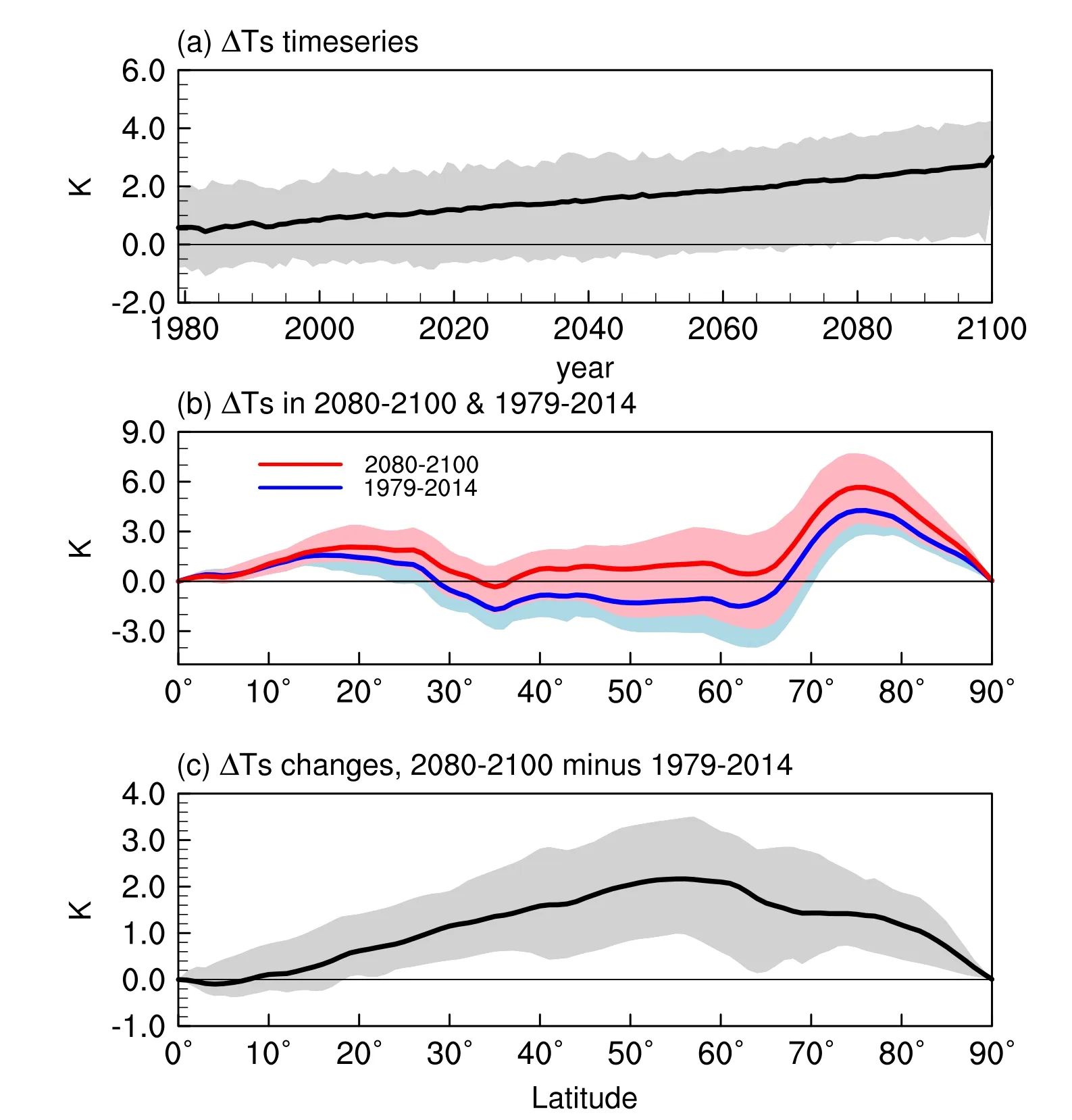
Fig.8.Projected changes in interhemispheric surface temperature contrast in the 21st century simulated by historical and SSP5-8.5 simulations: (a) time series from 1979 to 2100;(b)latitudinal distribution of interhemispheric surface temperature difference (weighted by the cosine of latitude) for the (blue) 1979-2014 and (red) 2080-2100 mean;(c) latitudinal distribution of the changes in interhemispheric surface temperature contrast (weighted by the cosine of latitude).Changes are calculated as the difference between 2080-2100 and 1979-2014.The blue/red/gray shading marks the intermodel spread.

Figures 9a-e show the means of and changes in the interhemispheric warming asymmetry and contributions from the interhemispheric SW/Gcontrast and the cross-equatorial OHT/AHT,respectively.Compared with the climatology of the two periods (crosses in Fig.8),it shows that the interhemispheric temperature contrast will increase by～1.8 K for the CMIP6 mean.This increase is caused by the increases in interhemispheric SW contrast (～0.6 K),as well as the increase in interhemisphericGcontrast (～1.5 K).While the reduced northward OHT acts to reduce the interhemispheric surface temperature contrast (around -0.3 K),the contributions from the cross-equatorial AHT changes can be ignored(around -0.1 K).

The magnitude of the interhemispheric warming asymmetry shows a large range among different models (bar charts in Fig.9a).The interhemispheric temperature contrast is projected to increase by 0.9 K in IITM-ESM and by 2.7 K in CanESM5.Note that the order of models in Fig.9 has changed compared to Fig.3,indicating that the interhemispheric warming asymmetry is independent of the model performance regarding the climatological interhemispheric temperature contrast.

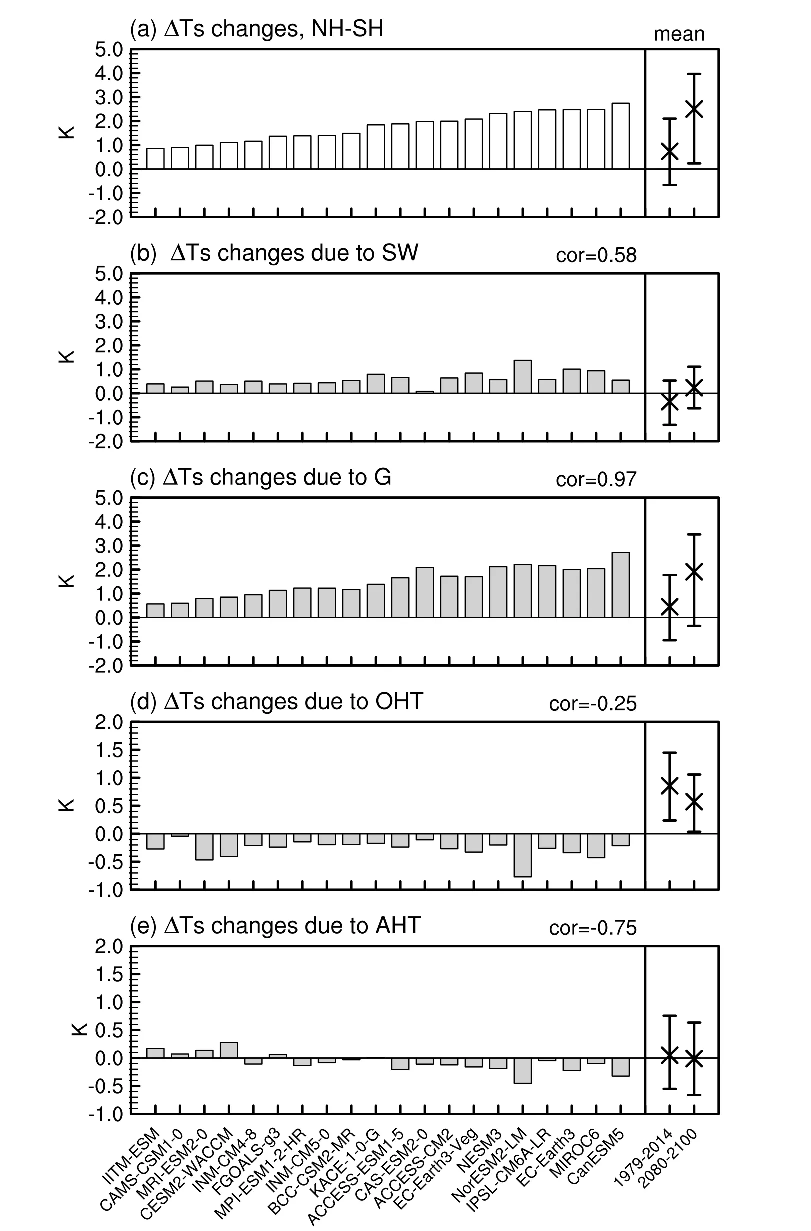
Fig.9.Means and changes of interhemispheric surface temperature contrast and contributions from different processes: (a) interhemispheric surface temperature contrast;(b) contribution of interhemispheric SW contrast;(c) contribution of interhemispheric G contrast;(d) contribution of cross-equatorial OHT;(e) contribution of cross-equatorial AHT.Bar charts on the left show the changes between 2080-2100 and 1979-2014.Black crosses on the right show the multimodel ensemble mean’s climatology in each period,and error bars show the minimum and maximum values of the climatology among all models.

Fig.10.Projected precipitation changes in the 21st century.Changes are calculated as the difference between the 2080-2100 mean (in SSP5-8.5 simulations) and 1979-2014 mean (in the historical mean): (a) maps of multimodel mean precipitation changes,in which contours represent the climatological mean of 1979-2014 (interval: 2 mm d-1)and dotted regions indicate precipitation changes that are statistically significant at the 95% confidence level(Student’s t-test);(b) latitudinal distribution of zonal mean precipitation during 1979-2014 (solid black line),2080-2100 (dashed black line),and the projected changes (red line);(c) scatter plot of the tropical precipitation asymmetry index (PAI) changes versus the interhemispheric warming asymmetry,in which the cross marks the multimodel mean changes.

Among the four processes,the intermodel spread of the interhemispheric warming asymmetry is positively related to the change inG(Fig.9c,r=0.97) and SW (Fig.9b,r=0.58),but negatively related to the change in AHT (Fig.9e,r=-0.75).There is a weak correlation between the intermodel spread in the interhemispheric warming asymmetry and the changes in cross-equatorial OHT.These results confirm the important role of changes in interhemisphericGand SW contrast in causing interhemispheric warming asymmetry.The details of the changes inGand SW are not analyzed because the above analysis shows that the uncertainty in these future changes is independent of model performance regarding the climate mean state,which is an important issue beyond the scope of this paper.The possible factors of influence are discussed in section 4.

Figures 10a and b show the CMIP6 mean projected precipitation changes by the end of this century.In the deep tropics (10°S-10°N),there are significant increases in precipitation over the equatorial Pacific,Atlantic,and western Indian Ocean.Over the subtropics (15°-30°S/N),the precipitation changes show an obvious pattern of interhemispheric asymmetry,with increases in precipitation in the NH but decreases in the SH.Figure 9c shows that the tropical PAI will increase in association with the interhemispheric warming asymmetry.These two indices have a significant crossmodel positive correlation (r=0.55),indicating that the tropical precipitation will increase more to the north of the equator in association with the stronger NH warming.This suggests that the changes in interhemispheric temperature contrast are of significant importance in modulating the tropical precipitation changes and the latitudinal displacements of the ITCZ.These results are consistent with previous findings reported by Friedman et al.(2013) and Geng et al.(2022).

4.Discussion and conclusions

The performances of 26 CMIP6 models in simulating the climatological interhemispheric surface temperature contrast were studied.We quantified model biases of interhemispheric surface temperature contrast based on the energy balance assumption,and the results highlight the importance of cloud bias in AGCMs in causing biases in interhemispheric surface temperature contrast.The main conclusions from our study can be summarized as follows:

Compared with reanalysis datasets,most CMIP6 models underestimate the interhemispheric surface temperature contrast between the NH and SH.The interhemispheric surface temperature contrast ranges from -0.7 K to 2.3 K,with a multimodel mean of 0.8 K,compared to a mean value of～1.4 K in the Reanalysis-1 and ERA5 datasets.The underestimation of the interhemispheric surface temperature contrast in CMIP6 models is in agreement with the findings of previous studies based on CMIP5 models.For example,the warm SST bias in the SH (Wang et al.,2014;Xu et al.,2014;Găinuşă-Bogdan et al.,2018) and cold SST (Wang et al.,2014) and surface temperature bias in the NH (Levine et al.,2013).This implies that further efforts are needed to improve the simulation of the interhemispheric temperature contrast.

Using a simple box model according to the energy balance of each hemisphere,it is shown that the underestimated interhemispheric contrast in SW andG,as well as the underestimated cross-equatorial northward OHT,all contribute to the underestimation of the interhemispheric surface temperature contrast.In quantitative terms,the contributions from SW,Gand OHT are -0.6 K,-0.8 K and -0.4 K,respectively.The cross-equatorial southward AHT is also underestimated in CMIP6,leading to an increase in the interhemispheric temperature contrast of 1.2 K compared with that in the reanalysis datasets.As a result,the CMIP6 mean underestimates the interhemispheric temperature contrast by about-0.6 K.

Comparing between models,we find that the intermodel spread in the interhemispheric temperature contrast can be traced back to biases in the midlatitude cloud properties in AGCMs.Models with negative interhemispheric surface temperature contrast biases tend to underestimate the cloud SW reflection in the SH,while overestimating it in the NH.The negative cloud SW reflection bias is likely related to the underestimation of cloud cover over the SH midlatitude ocean,and the positive cloud SW reflection bias is likely related to the overestimation of cloud liquid water content over the NH midlatitude continents.Simulated cloud errors have been considered as important sources of model uncertainty (Hwang and Frierson,2013;Su et al.,2013;Dolinar et al.,2015;Mechoso et al.,2016;Hu et al.,2017;Fan et al.,2018;Miao et al.,2021).Further in-depth studies are needed to elucidate the specific underlying mechanisms involved,including details of ice cloud parameterizations(Ma et al.,2012),stratiform cloud schemes (Geoffroy et al.,2017),and convection schemes (Lin,2019).

There are increasing trends in the interhemispheric surface temperature contrast until the end of the 21st century.The box model results show that the increase in interhemispheric surface temperature contrast (～1.8 K) is caused by the increase in interhemisphericGcontrast (～1.5 K) and SW contrast (～0.6 K).The reduced northward OHT acts to reduce the interhemispheric surface temperature contrast(approximately -0.3 K),and the contribution from the crossequatorial AHT changes is -0.1 K and can be ignored.The increasing interhemisphericGcontrast may be partly due to there being larger continental areas over the NH,and the continents having a larger greenhouse trapping effect than the ocean (Kang et al.,2015).The increasing interhemispheric SW contrast is likely related to the reduction in Arctic sea ice (Holland et al.,2006) and the globally uneven increase in anthropogenic aerosols (Bellouin et al.,2020).The source of uncertainty in the future interhemispheric warming asymmetry is independent of model performance with respect to the climatological interhemispheric temperature contrast.Further investigation is needed to clarify the effects of the intermodel spread in future changes in sea ice,ocean circulation and heat content,clouds and aerosols in modulating future interhemispheric warming asymmetry.

Acknowledgements.This work was supported by the National Natural Science Foundation of China (Grant No.41888101).The outputs from CMIP6 can be download from https://esgf-node.llnl.gov/projects/cmip6/.The NCAR-NCEP (Reanalysis-1) data can be download from https://psl.noaa.gov/data/reanalysis/reanalysis.shtml.The ERA5 data can be download from https://www.ecmwf.int/en/forecasts/datasets/reanalysis-datasets/era5.