Assimilation of GOES-R Geostationary Lightning Mapper Flash Extent Density Data in GSI 3DVar,EnKF,and Hybrid En3DVar for the Analysis and Short-Term Forecast of a Supercell Storm Case

Rong KONG,Ming XUE,Edward R.MANSELL,Chengsi LIU,and Alexandre O.FIERRO

1Center for Ana-lysis and Prediction of Storms, Norman Oklahoma 73072, U.S.A.

2University of Oklahoma, Norman Oklahoma 73072, U.S.A.

3NOAA/National Severe Storms Laboratory, Norman, Oklahoma 73072, U.S.A.

4Zentralanstalt für Meteorologie und Geodynamik, Department of Forecasting Models -ZAMG, Vienna 1190, Austria

ABSTRACT Capabilities to assimilate Geostationary Operational Environmental Satellite “R-series” (GOES-R) Geostationary Lightning Mapper (GLM) flash extent density (FED) data within the operational Gridpoint Statistical Interpolation ensemble Kalman filter (GSI-EnKF) framework were previously developed and tested with a mesoscale convective system(MCS) case.In this study,such capabilities are further developed to assimilate GOES GLM FED data within the GSI ensemble-variational (EnVar) hybrid data assimilation (DA) framework.The results of assimilating the GLM FED data using 3DVar,and pure En3DVar (PEn3DVar,using 100% ensemble covariance and no static covariance) are compared with those of EnKF/DfEnKF for a supercell storm case.The focus of this study is to validate the correctness and evaluate the performance of the new implementation rather than comparing the performance of FED DA among different DA schemes.Only the results of 3DVar and pEn3DVar are examined and compared with EnKF/DfEnKF.Assimilation of a single FED observation shows that the magnitude and horizontal extent of the analysis increments from PEn3DVar are generally larger than from EnKF,which is mainly caused by using different localization strategies in EnFK/DfEnKF and PEn3DVar as well as the integration limits of the graupel mass in the observation operator.Overall,the forecast performance of PEn3DVar is comparable to EnKF/DfEnKF,suggesting correct implementation.

Key words: GOES-R,lightning,data assimilation,EnKF,EnVar

1.Introduction

High spatiotemporal resolution lightning data offer a reliable complement to radar data that can be assimilated into convection-allowing NWP models,especially in regions where the Next-Generation Radar (NEXRAD,Doviak et al.,2000) Weather Surveillance Radar-1998 Doppler (WSR-88D) radar coverage is poor or absent,such as in mountainous areas due to beam blockage,or in oceanic regions beyond the range of ground-based radars.Efforts have been made to assimilate lightning data into convection-allowing NWP models using nudging (e.g.,Fierro et al.,2012,2015;Marchand and Fuelberg,2014),3DVar (Fierro et al.,2016,2019;Hu et al.,2020),4DVar (Xiao et al.,2021),and EnKF methods(Mansell,2014;Allen et al.,2016).Results show that the assimilation of either cloud-to-ground (CG) and especially total (CG plus intra-cloud) lightning data often produces forecast improvements comparable to those from assimilating ground-based radar data (Fierro et al.,2016).Among these studies,Mansell (2014) assimilated explicitly-simulated flash extent density (FED) data,and Allen et al.(2016) assimilated pseudo-geostationary lightning mapper (GLM,Goodman et al.,2013) observations derived from ground-based lightning mapping array (LMA,Rison et al.,1999;MacGorman et al.,2008) data,both using the more advanced ensemble Kalman filter (EnKF,Evensen,1994) method.Here,FED is a type of lightning flash rate and can be concisely defined as the total number of lightning flashes occurring within a given atmospheric column over a specified period(Lojou and Cummins,2005).The readers are referred to Bruning et al.(2019) for more information on the derivation of GLM FED data.Observation operators for FED that depend on graupel echo volume or graupel mass were developed,based on output data from storm-scale simulations conducted with explicit electrification physics (Mansell et al.,2002,2005;Allen et al.,2016).With these observation operators,the FED is linearly related to the total graupel mass or graupel volume within the FED pixel column.Other studies by Fierro et al.(e.g.,Fierro et al.,2012),Marchand and Fuelberg(2014),and Qie et al.(2014) assimilated some form of pseudo-data (water vapor mass,temperature,or ice-phase particles) derived from the lightning data either through nudging or 3DVar,and such assimilation was shown to improve convective initialization and short-term forecasts.

The GLM instruments on the GOES-R series geostationary satellites detect the light emitted by lightning at the cloud tops and collect information about total lightning discharges (Goodman et al.,2013).The GOES-R GLM is able to continuously detect total lightning activity (intra-cloud plus CG) over the Americas and adjacent oceanic regions with a spatial resolution/footprint ranging from 8 km near the center of the field of view (near nadir) to about 12 km near the edges.GLM records information such as the frequency,location,optical energy,and extent of light emitted from lightning discharges to better depict the presence of developing and intensifying thunderstorms.NOAA/NASA maintains two GOES-R series operational geostationary satellites: GOES-16 in the GOES-East position and GOES-17 in the GOES-West position.Operational datasets from these satellites have been made available since late 2017 and early 2019,respectively.In March 2022,GOES-18 was launched into space and went into operational service as GOES-West on 4 January 2023,replacing GOES-17.

Recently,real GLM lightning observations have been successfully assimilated [e.g.,Fierro et al.(2019),Hu et al.(2020),and Kong et al.(2020)].Fierro et al.(2019) and Hu et al.(2020) used indirect assimilation of lightning (flash density rates) through pseudo-observations for water vapor mass,as derived from GLM lightning observations with a 3DVar system (Gao et al.,2016;Wang et al.,2018).Kong et al.(2020) assimilated GLM lightning (flash extent data)more directly using an EnKF method.In Fierro et al.(2019),the added value of lightning DA was investigated by assimilating Level II radar data with and without GLM-derived water vapor pseudo-observations for a group of severe convective storms.The GLM and radar assimilation experiments yielded short-term forecast improvements that were superior to those of a control run assimilating no data,with results on a par with previous studies assimilating pseudo-GLM observations (Fierro et al.,2015,2016).

Kong et al.(2020) was the first study to use an EnKF method to directly assimilate real GOES-R lightning observations.In their proof-of-concept study,the capabilities to assimilate GLM FED data were implemented into the NCEP operational EnKF DA system (Gridpoint Statistical Interpolation,GSI,Kleist et al.,2009a) and tested for a mesoscale convective system (MCS).FED observation operators based on graupel mass or graupel volume were used,and the results were compared to a control experiment that did not assimilate any data.The direct assimilation of FED observations was shown to noticeably improve the analysis and prediction of the MCS for up to several hours.Akin to the indirect methods,EnKF FED DA is effective in identifying and properly initializing regions of intense convection,which helps improve shorter-term forecasts of high-impact convective events.Direct and indirect adjustments to graupel and other model state variables through the ensemble covariances helped produce more balanced analyses and,thus,improved forecasts.

EnKF methods derive background error covariance from an ensemble of forecasts.The hybrid ensemble-variational (EnVar) DA technique employs a combination of ensemble-derived covariances and static covariances (typically used in 3DVar) to help alleviate the problems with covariance matrix rank deficiency and other issues (Hamill and Snyder,2000;Lorenc,2003;Etherton and Bishop,2004;Buehner et al.,2010).Hybrid EnVar capabilities have been implemented within the NCEP operational GSI (Kleist et al.,2009b) DA framework and are used operationally in the Global Data Assimilation System (GDAS,Hamill et al.,2011;Kleist and Ide,2015),the regional North American Mesoscale (NAM) Data Assimilation System (Wu et al.,2017),and the Rapid Refresh (RAP,Benjamin et al.,2016)DA system (Pan et al.,2014;Hu et al.,2017).For both the NAM and RAP,the operational EnVar DA systems borrow ensemble perturbations from the GDAS EnKF although coupling EnVar with one’s own EnKF system is most desirable and has been tested earlier for prototype RAP configurations(Pan et al.,2014,2018;Pu et al.,2016;Lu et al.,2017).

An earlier effort geared toward lightning data assimilation (LDA) using the hybrid ensemble-variational DA method can be found in Apodaca et al.(2014).In their study,pseudo-GLM data (derived from the ground-based lightning network) was assimilated using a hybrid EnVar DA method and applied to mesoscale models in which deep convection cannot be explicitly resolved.Their operator started with an approximate calculation of vertical velocity obtained from the Nonhydrostatic Mesoscale Model core of the Weather Research and Forecasting system (WRF-NMM),using a reduced version from the nonhydrostatic continuity equation.Although the operator can analyze some updrafts that are linked to other state variables through the continuity equation,the relative coarser grid resolution (e.g.,9 km in their study) is not suitable for convective scale DA.

Toward the eventual goal of operational implementation at NCEP,the convective-scale EnKF DA capability for GLM FED data in Kong et al.(2020) was implemented within the operational GSI EnKF framework.Given that hybrid EnVar is the current method of choice for the two operational regional forecasting systems (NAM and RAP),it is naturally desirable to implement and test hybrid EnVar DA capability for FED data within the GSI framework.This study aims at validating the correctness and evaluating the performance of the new implementation.In contrast to EnKF,EnVar obtains its analysis by minimizing a cost function,as in 3DVar.In fact,it builds upon the GSI 3DVar framework using the extended control variable algorithm of Lorenc(2003).The 3D version of EnVar is referred to as En3DVar(Liu and Xue,2016).

Specifically,this study includes three overarching goals:1) to implement GLM FED DA capabilities into the operational GSI EnVar that is coupled with GSI EnKF,2) to compare the performances of FED DA using EnKF and En3DVar to see whether comparable results can be obtained between En3DVar and EnKF,and 3) to evaluate the benefit of FED DA to short-range forecasts of a supercell storm case.Apart from lightning and precipitation,we also evaluate the ability of FED DA to improve the updraft helicity track forecast for the supercell storm case,which is commonly used as a proxy for tornado prediction in operational centers(Kain et al.,2008;Sobash et al.,2016).

2.Assimilation methods and procedures

2.1.The EnKF and DfEnKF algorithm

The EnKF within GSI uses a scalable implementation of the ensemble square root filter (EnSRF,Whitaker and Hamill,2002),which updates state variables and pre-calculated observation priors independently (Anderson and Collins,2007).The scalable implementation is equivalent to the traditional algorithm that updates state variables and recalculates observational priors when using linear observation operators,and it can produce qualitatively similar results as the traditional EnKF for practical NWP applications (Anderson and Collins,2007).For more detailed information about the updating equations of the GSI EnKF algorithm,the reader is referred to Kong et al.(2020).

To facilitate a more direct comparison between EnKF and pure En3DVar (PEn3DVar) that uses 100% ensemble covariance (as in EnKF),a deterministic EnKF (DfEnKF)algorithm,introduced by Kong et al.(2018),is also adopted here.In DfEnKF,an additional deterministic forecast (separate from the ensemble members) is updated using the same EnKF equation that is used to update the ensemble mean.The updated state becomes the initial condition for the deterministic forecast of the next cycle.The En3DVar is a deterministic algorithm as well;it updates a single background forecast variationally,utilizing the same ensemble perturbations as DfEnKF from a (one-way) coupled EnKF system(e.g.,Fig.1 of Pan et al.,2014).Given that pure En3DVar is one-way coupled with the EnKF,as is DfEnKF,the results between PEn3DVar and DfEnKF could be similar but not necessarily the same.First,for EnKF/DfEnKF,observations are assimilated serially (one after another),while for PEn3DVar,all observations are assimilated globally (at the same time).Analyses could be different when the observation operator is nonlinear.Second,for EnKF and DfEnKF,localizations are conducted between the model and the observation space,while for En3DVar,localizations are conducted purely in the model space.

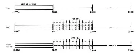
Fig.1.Flow diagram of the EnKF (middle),3DVar,and DfEnKF and En3DVar (bottom) DA experiments versus the control run (top).The spin-up ensemble forecasts from 2100 UTC through 2200 UTC include 40 members.FED DA occurs between 2200 and 2300 UTC with 5-minute cycles,and a deterministic forecast is launched from the final ensemble mean analysis at 2300 UTC and runs to 0500 UTC.The CTRL experiment continues the ensemble forecasts through 2300 UTC without DA,and a single deterministic forecast continues from the ensemble mean forecast at 2300 UTC.

2.2.The En3DVar algorithm

The hybrid En3DVar algorithm based on the extended control variable method of Lorenc (2003) is used in GSI,in which the full-rank static background error covariances and the rank-deficient ensemble covariances are combined through the introduction of a set of extended control vectors.The analysis increment is given by

where δx1and δx2are the analysis increments related to the static and ensemble background error covariances,respectively.

where 1/β1and 1/β2are the weights given to the static and ensemble background error covariances,respectively.A hybrid solution is derived by setting 1/β1or 1/β2to values between 0 and 1.B is the static background error covariance matrix and A is the matrix used to localize the ensemble background error covariance.d is the observation innovation vector,H is the linearized observational operator,and R is the(diagonal) observation error covariance matrix.When the weight for the static (ensemble) background error covariance is 0,the hybrid algorithm degenerates to pure En3DVar(pure 3DVar).

In this study,temperature-dependent background error profiles for hydrometeor mixing ratios,proposed by Liu et al.(2019),are adopted when constructing the static background error B to generate more reasonable graupel increments.

As in Kong et al.(2018),the hybrid En3DVar system is one-way coupled with EnKF;noting that with one-way coupling,it is easier to separate En3DVar from EnKF when comparing their relative performance and understanding their respective behaviors.In general,little difference is expected between one-way and two-way coupled EnKF-En3DVar when the DA cycles are run for a short period (Pan et al.,2014).For long,continuously cycled DA systems,however,two-way coupling is strongly recommended since divergence between the EnKF and En3DVar systems can occur with time in a one-way coupling mode (Pan et al.,2014).

2.3.The FED observation operator

The tuned FED observation operator used in this study is based on graupel mass instead of graupel echo volume[Kong et al.(2020)].The graupel-volume-based FED observation operator cannot be easily used in a variational framework,because of the zero gradient of the cost function that is realized when differentiated with respect to the graupel mixing ratio.This is because the graupel volume is no longer sensitive to the graupel mixing ratio once its value exceeds the threshold (e.g.,0.5 g kg-1) used to define the graupel volume.The FED observation operator based on graupel mass(GM in kg) from Kong et al.(2020) is given by

This operator has been tuned through sensitivity experiments and the coefficient has been multiplied by a factor of 0.5 compared to the original operator used in Allen et al.(2016).Similar to Mansell (2014) and Allen et al.(2016),the graupel mass within each grid cell is summed over a volume spanning the vertical depth of the model and covering a 15×15 km2horizontal area that is centered on the observation pixels,so that the lightning occurring in the vicinity of a typical GLM pixel (8×8 to 12×12 km2) can be accounted for.

Through the observation operator,information on lightning observations can be transferred in the variational analysis to the graupel mixing ratio due to its direct linkage with the FED observations.Other state variables (water vapor mixing ratio,temperature,vertical velocity,etc.) are linked through the ensemble-derived background error covariances.When a pure static background error covariance is used in 3DVar,only the graupel mixing ratio is directly updated by FED observations (due to lacking cross-variable correlations in the static background error covariance B),although other state variables can respond to the FED DA during the forecast period through either microphysical or thermodynamical adjustments.

The implementation of the FED observation operator involves the integration of the graupel mass field over a fixed area (15×15 km2in our case) centered on the observation.The number of model columns being used for integration is determined adaptively based on model resolution.For example,a 5×5 region would be used for horizontal integration on a 3-km model grid and 15×15 for the 1-km model grid used here.

3.Simulation setup and experimental design

3.1.GOES-R GLM-FED data and their processing

The FED observations were derived from the GOES-16 level-2 GLM data,which are provided in 20-sec packets with an 8-12 km pixel resolution over the contiguous United States (CONUS,Goodman et al.,2013).The level-2 data include three different primary lightning metrics -i.e.,the flashes,groups,and events -which are governed by specific parent-to-child relationships (Goodman et al.,2013;Bruning et al.,2019).Similar to Kong et al.(2020),the lightning observations are mapped onto 10-km grid pixels to obtain the FED observations,with the number identification of the groups and flashes being tracked to each matching event.The number of events is directly used to calculate the FED,which by definition increases by increments of one for each flash on each pixel (in contrast to flash source densities).More details on the FED data processing can be found in Kong et al.(2020).

3.2.Forecast model setup and initialization of ensembles

The Advanced Research WRF (ARW) model is used in this study,which is a three-dimensional compressible nonhydrostatic NWP model (Skamarock et al.,2008).The model uses a 600×600 grid with 1-km horizontal grid spacing on a single domain and has 53 stretched vertical grid levels with a model top set at about 21 km.

Similar to the configurations of Kong et al.(2020),40 initial ensemble members are generated based on the deviations of the 2100 UTC analyses of the NCEP operational Short-Range Ensemble Forecast system (SREF,which has 26 members with a 16-km horizontal resolution) from the 3-h North American Model (NAM) forecast (with a 12-km horizontal grid spacing) valid at the same time.The deviations are reduced by 25% (determined through experimentation),and their negative versions are combined to produce a total of 40 perturbations.Following Tong and Xue (2008),Snook et al.(2012),and Johnson et al.(2014),added a set of additionally smoothed small-scale random perturbations with a Gaussian distribution to the horizontal components of the wind field,potential temperature,and humidity fields to introduce convective-scale perturbations.The initial ensembles are then advanced one hour to 2200 UTC,with the same surface and boundary parameterizations and 6-class Thompson bulk microphysical scheme (Thompson et al.,2008).More details on the physics options can be found in Kong et al.(2020).

3.3.Design of data assimilation experiments

As mentioned in section 2c,the graupel-mass-based observation operator from Kong et al.(2020) was used in this study.The assimilation of GLM FED data using 3DVar,EnKF,and pure En3DVar methods are evaluated against each other.Their results are also compared with a control experiment (CTRL) that does not assimilate any data.Since the purpose of this study is to validate the correctness of the implementation of FED DA within the GSI variational DA framework,only 3DVar and pure En3DVar (instead of hybrid En3DVar) are tested.More detailed information about different DA experiments is provided in Table 1.

Table 1.Descriptions of the DA experiments.

FED observations are assimilated in 5-min intervals over a 1-h period in all DA experiments as in Kong et al.(2020).To help suppress spurious storms in the background,zero FED observations are also assimilated.A 0.95 adaptive posterior inflation that relaxes the posterior spread to the prior spread (Whitaker and Hamill,2012;Kotsuki et al.,2017;Maldonado et al.,2020) is used to help maintain ensemble spread.The FED operator is a vertical integral of graupel mass,and,like the GLM FED observations,has no inherent vertical location.Nevertheless,we need to specify the height of the FED observation for vertical covariance localization in EnKF (which uses observation-space localization).The FED observation is assigned to an assumed height of 6.5 km in the EnKF (Allen et al.,2016;Kong et al.,2020),which generally falls within the mixed-phase region where most lightning is initiated.This is not needed in En3DVar because localization is conducted in the model instead of observation space.Similar to Allen et al.(2016) and Kong et al.(2020),the horizontal and vertical localization radii in the EnKF are set to 15 km and -4 in log(P/Pref) space(～32 km on average).With the large vertical localization radius,there is effectively no vertical localization,and the FED observations are allowed to influence the whole vertical depth.The actual spatial spreading of analysis increments is governed by the ensemble covariance (Kong et al.,2020).This is confirmed by a single observation experiment,where results are found to be insensitive to the specified height of the FED observation (results not shown).In 3DVar and hybrid En3DVar,the decorrelation length scale for the static background error covariancesBis set to 6 km in the horizontal and to 1.5 grid points in the vertical (tuned through experiment),which are larger than those used in Hu et al.(2020).Because the graupel mass observation operator is integrated over a 15×15 km2column,the FED observation does influence a much larger area than that implied by the decorrelation length scale ofB.The horizontal and vertical decorrelation length scales used to localize the ensemble covariances in En3DVar are 4.1 km and -1.1 inlog(P/Pref)space,respectively,which are equivalent to the cut-off radii of 15 km and -4 in log(P/Pref) used in EnKF based on Pan et al.(2014).Considering that the flash rates from the GLM are overall smaller than those detected by very-high frequency ground-based LMA (Rison et al.,1999) networks for highflash-rate storms (Carey et al.,2019),a small observation error of 0.5 flashes min-1pixel-1is used in this study [as in Kong et al.(2020)].Moreover,initial sensitivity experiments revealed that setting an observation error smaller than 0.5 flash min-1pixel-1can result in observation overfitting and numerical instability during model integration.

For the DA experiments,the first analysis is made at 2200 UTC 1 May 2018,or 1 h into the spinup ensemble forecasts from the perturbed initial conditions (Fig.1).After the 1-h DA period,a 6-h forecast is made from the final analysis to examine the impact of lightning DA on storm forecasts.

3.4.Case overview

A severe weather event occurred in north central Kansas and southern Nebraska in the afternoon and evening of 1 May 2018.Multiple supercells spawned nearly a dozen tornadoes,including a long-track EF-3,across the state of Kansas.The storms were mainly influenced by a stationary front over north-central Kansas (Figs.2a-d),with favorable wind shear and cold air aloft coupled with an abundant supply of low-level moisture advected from the Gulf of Mexico by a low-level jet.A dryline extending southward from the stationary front across west-central Kansas also triggered scattered thunderstorms.The convective inhibition (CIN) values of the 1200 UTC and 1900 UTC soundings from the NWS site of Dodge City,Kansas (DDC) were 253 J kg-1and 4 J kg-1,respectively.The changes in boundary-layer thermodynamics (reduction in inhibition via erosion of the cap by solar heating) coupled with a progressive destabilization of the environment (60 hPa mixed layer CAPE at 1900 UTC exceeding 2000 J kg-1) allowed some cumulus turrets to develop along the stationary front and along portions of the dry line in central Kansas.At 2100 UTC,a line of semi-discrete storms developed along the stationary front (Fig.2a).These cells within the line progressively moved eastward while intensifying into severe-warned storms by 2200 UTC(Fig.2b).Our DA focuses on the period with frequent lightning activity between 2200 UTC to 2300 UTC 1 May.Isolated supercell storms developed over the next few hours,producing several tornadoes,strong wind events,and reports of hail up to the size of softballs (10-cm diameter).

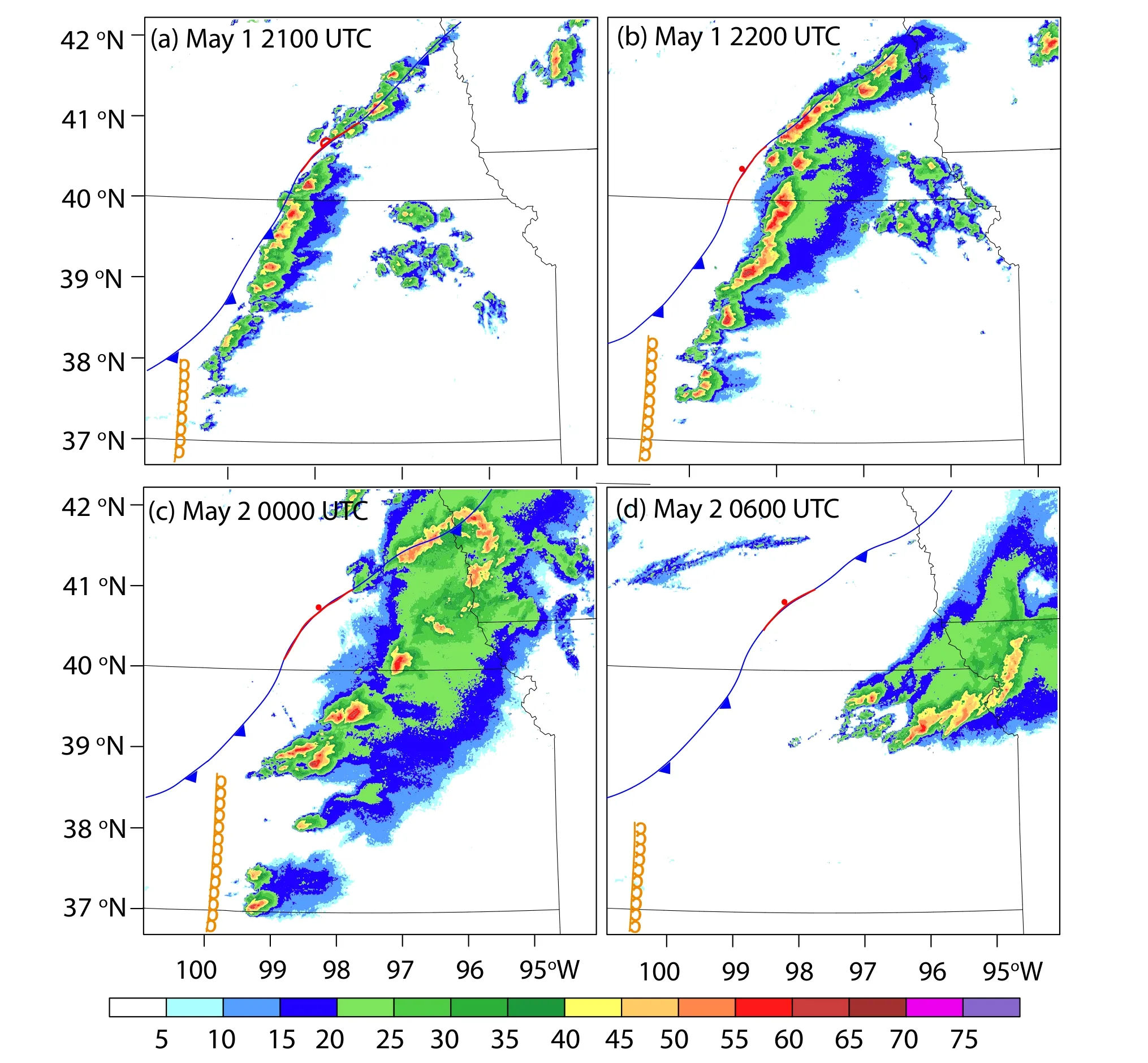
Fig.2.Locations of the fronts [reproduced based on the surface analysis from the storm prediction center (SPC)],overlaid with the composite reflectivity observations (dBZ) remapped from the WSR-88D radars (shaded contour) on(a) 2100 UTC 1 May,(b) 2200 UTC 1 May,(c) 0000 UTC 2 May,and (d) 0600 UTC 2 May 2018,respectively.

4.Results

4.1.Convergence of the 3DVar/En3DVar cost function and computational costs of different DA methods.

The convergence of the quadratic cost function is evaluated first to validate the correctness of the FED DA procedure in the variational DA framework.Since the observation operator is linear,the double-loop procedure that is usually used to linearize a nonlinear observation operator (such as for reflectivity) is not needed here.Only one outer loop (with 50 maximum iterations) is used in this study.Figure 3a shows the value of the cost function as a function of iterations in the first FED DA cycle for both cases.Pure 3DVar converges slightly faster than PEn3DVar.Overall,15 iterations are sufficient for convergence in both 3DVar and PEn3DVar.In our study,50 iterations are used for all the variational DA experiments to secure convergence of the cost function.

The computational costs of different DA schemes are also compared in Fig.3b.Overall,the computation cost of EnKF is 60% higher than 3DVar and both are much lower than PEn3DVar,for which the cost function evaluation and minimization consume most of the computational time.The EnKF computation/analysis is performed in the observational space,and thus the computational cost is proportional to the number of observations.The observational density of the two-dimensional FED data is much less than the three-dimensional radar data.If FED data are assimilated together with 3D radar data in EnKF,the additional cost incurred by the FED DA becomes negligible.For EnVar,the computational cost is proportional to the length of the state vector,which includes the much larger extended state vectorα[see Eq.(2)].

Fig.3.(a) Value of the cost function as a function of iteration loops for both the 3DVar and PEn3DVar runs (there is only one outer loop,with 50 iterations in the loop) in the first analyses and (b) the computational cost (wall time in seconds) of 3DVar,EnKF,and PEn3DVar.

4.2.Single-point observation experiment

To demonstrate the direct impacts of lightning DA on the analyses of hydrometeor fields,single point experiments(with grid columnx=230,y=360 being the closet to the center of the single observation pixel) are conducted and compared between DfEnKF and pure En3DVar that uses 100% ensemble covariance (PEn3DVar).Vertical cross-sections of the analysis increments [ xa-xbin Eq.(1)] for the mixing ratios of rain,snow,and graupel are made through the single observation point.As in Kong et al.(2020),the horizontal localization radius for the DfEnKF is 15 km (15 km is the zero point) and the vertical localization scale is 4 in logPspace.Since the vertical localization radius is very large (about 32 km on average in the vertical),the effective vertical location is not considered in our DA experiments.To ensure similar localization scales being used in both PEn3DVar and EnKF,equivalent recursive filter length scales based on Pan et al.(2014) are used for localization,which is about 4.11 km in horizontal and 1.10 in logPspace for PEn3DVar.

As shown in Fig.4,the magnitude and horizontal extent of the analysis increment of the hydrometeors of graupel,snow,and rainwater for PE3DVar (Fig.4b) are much larger than DfEnKF (Fig.4a).The differences in the analysis increments probably arise from the localization and the volume integration of the graupel mass in the observation operator.To eliminate the influence caused by horizontal integration of the graupel mass in the FED observation operator,the horizontal integration is arbitrarily turned off and the vertical integration remains unchanged.In other words,the integration is conducted only over a single grid column with a 1×1 km2area and multiplied by a factor of 15^2 (i.e.,the full area) to achieve a similar physical meaning as the original operator.The observation operator is only modified to help understand the problem,and the original version was used for the experiments discussed in the following sections.After turning off the horizontal integration in the observation operator,the horizontal extension of the analysis increment from DfEnKF (Fig.4c) and PEn3DVar (Fig.4d) becomes very similar.Thus,the horizontal integration in the observation operator is the major cause for the difference in the analysis increment between DfEnKF and En3DVar under the influence of different localization strategies.

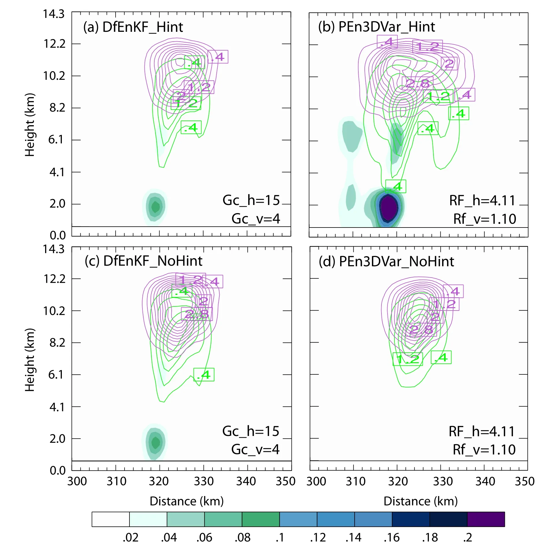
Fig.4.Vertical cross sections of the mixing ratio increments (g kg-1) of rain (shading,starting from 0.02 with 0.02 g kg-1 interval),snow (purple contours,start from 0.4 with 0.4 g kg-1 interval),and graupel (green contours,start from 0.4 with 0.4 g kg-1 interval) after the first analysis of (a,c) DfEnKF and (b,d) PEn3DVar using (a,b) the original observation operator and (c,d) the modified observation operator,respectively.The cross-section passes through the observation point (x=230 km,y=360 km).

4.3.Sensitivity of DfEnKF and En3DVar analyses to different localization scales

To further understand the impacts of the difference in localization and integration volume in the observation operator,sensitivity experiments are conducted to assimilate single FED observation with different horizontal and vertical localization scales.Unlike En3DVar,for which localization is conducted in the model space,EnKF needs the height information of the observation to conduct localization between the model and observation space.Following Allen et al.(2016)and Kong et al.(2020),the FED observations are assigned to a height of 6.5 km for DfEnKF DA.When the vertical localization radius is small (0.2 in logPspace),the difference between DfEnKF and PEn3DVar is most obvious.As is shown in Fig.5a,with a small vertical localization radius,the analysis increments of the graupel field for DfEnKF only exist in the levels around 6.5 km,while the analysis increment of PEn3DVar is more extended in vertical,since the localization of En3DVar is conducted in model space.When increasing the vertical location radius but keeping the horizontal localization the same,the difference between En3DVar and DfEnKF becomes smaller (Figs.5b,c,f,g).Furthermore,when the horizontal localization radius is increased to a very large value (e.g.,2000 km cutoff for DfEnKF),the difference between DfEnKF and PEn3DVar becomes very small.Without localization in both the horizontal and vertical directions,DfEnKF and PEn3DVar can obtain similar analysis increments (Figs.5d,h).

4.4.Comparisons of EnKF,DfEnKF,3DVar,and PEn3DVar

To evaluate how well the analyses match the observations after 1-h DA,the FED observation operator is applied to the final analysis of the DA experiments,and the simulated FEDs are compared with the FED observations.For the FED analyses after 1-h DA,EnKF,DfEnKF,and PEn3DVar are all able to better capture the observed discrete FED cores corresponding to the three main storm cells,which are more consistent with the observations than 3DVar or CTRL (Fig.6).The distribution of the FED field from CTRL is too linear and there are obvious location errors.3DVar produces a poorer FED analysis with more small-magnitude FEDs relative to EnKF,DfEnKF,and PEn3DVar as well as the observations,which is expected since 3DVar only updates the graupel field instead of the whole model state as in EnKF/DfEnKF and PEn3DVar during DA.

Fig.6.(a) 1-min FED observations (units: flash min-1 pixel-1) and FED forecasts from (b) CTRL;analyses (after 1-h DA)from (c) 3Dvar,(d) EnKF,(e) DfEnKF,and (f) PEn3DVar.

To quantitatively assess the performance of different DA experiments,the root-mean-square innovations (RMSI)of FED analyses and forecasts within the 1-h DA window and the follow-up 1-4 h FED forecasts for CTRL,3DVar,EnKF,DfEnKF,and PEn3DVar are displayed in Fig.7.Overall,EnKF performs best and has fewer spurious FED areas relative to the other DA methods (figure not shown).Within the DA cycles,taking the average of ensemble forecasts to obtain ensemble means can lead to weaker FED values,thus reducing the chance of overestimation (producing less spurious storms,figures not shown) in the EnKF analyses and forecasts relative to DfEnKF and PEn3DVar (which does not involve ensemble mean).3DVar has a smaller RMSI than CTRL during DA but increases quickly during the 1-h forecasts after the DA.The lack of consistent updating of all state variables is believed to be the main reason for this.

Fig.7.RMSIs of the FED forecasts (flash min-1 pixel-1) for CTRL;FED analyses and forecasts within the 1-h DA window,and 0-4 h free forecasts for 3DVar,EnKF,DfEnKF,and PEn3DVar,respectively.

Fig.8.5-km neighborhood ETSs of the supercell composite reflectivity analyses and forecasts verified against (a) 20 dBZ and (b) 35 dBZ within 1-h of DA (corresponding to -1 to 0 h after DA) and 0-4 h composite reflectivity forecasts after DA for experiments CTRL,3DVar,EnKF,DfEnKF,and PE3DVar,respectively.

To quantitively evaluate how well different DA experiments capture the structure and intensity of the storms,the 0-4 h forecasts of composite reflectivity fields from different experiments are verified against WSR-88D composite reflectivity using the equitable threat score (ETS;Mason,2003)with a 5-km neighborhood radius in Fig.8.For the threshold of 20 dBZ(Fig.8a),EnKF outperforms DfEnKF and PEn3DVar,apparently because EnKF generates fewer spurious storms than DfEnKF and PEn3DVar (figures not shown).Both DA methods produce overall better forecasts than 3DVar,which,in turn,still outperforms CTRL (in terms of ETS).For the threshold of 35 dBZ(Fig.8b),EnKF produces the best 0 to 1-h forecast.The ETSs of DfEnKF,PEn3Dvar,and 3DVar are similar and drop quickly during the first 0.5 h of the forecast.For 1 to 3 h,the DA experiments do not exhibit substantial improvements over CTRL.

Updraft helicity (UH;Kain et al.,2008) is an integrated measure of updraft rotation in supercells,and UH swaths have been shown to be a good proxy for tornado track forecasting (Clark et al.,2012).To evaluate how well different DA experiments predict rotating updrafts and tornadic potential,the accumulated swaths of the 2-5 km UH from the 0-2-hr forecasts of the velocity fields are compared with the locations of the official Storm Prediction Center (SPC) tornado and hail reports.As can be seen in Fig.9,EnKF,DfEnKF,and pure En3DVar perform similarly overall and outperform both the CTRL and 3DVar in terms of capturing the three different high UH swaths in southern Nebraska and north central Kansas that are consistent with the tracks of tornado and hail reports.The ensemble-based DA methods(EnKF/DfEnKF or En3DVar) all help improve the forecast location of rotating updrafts,and thus are able to provide more accurate prediction of potential severe weather threats for this case.

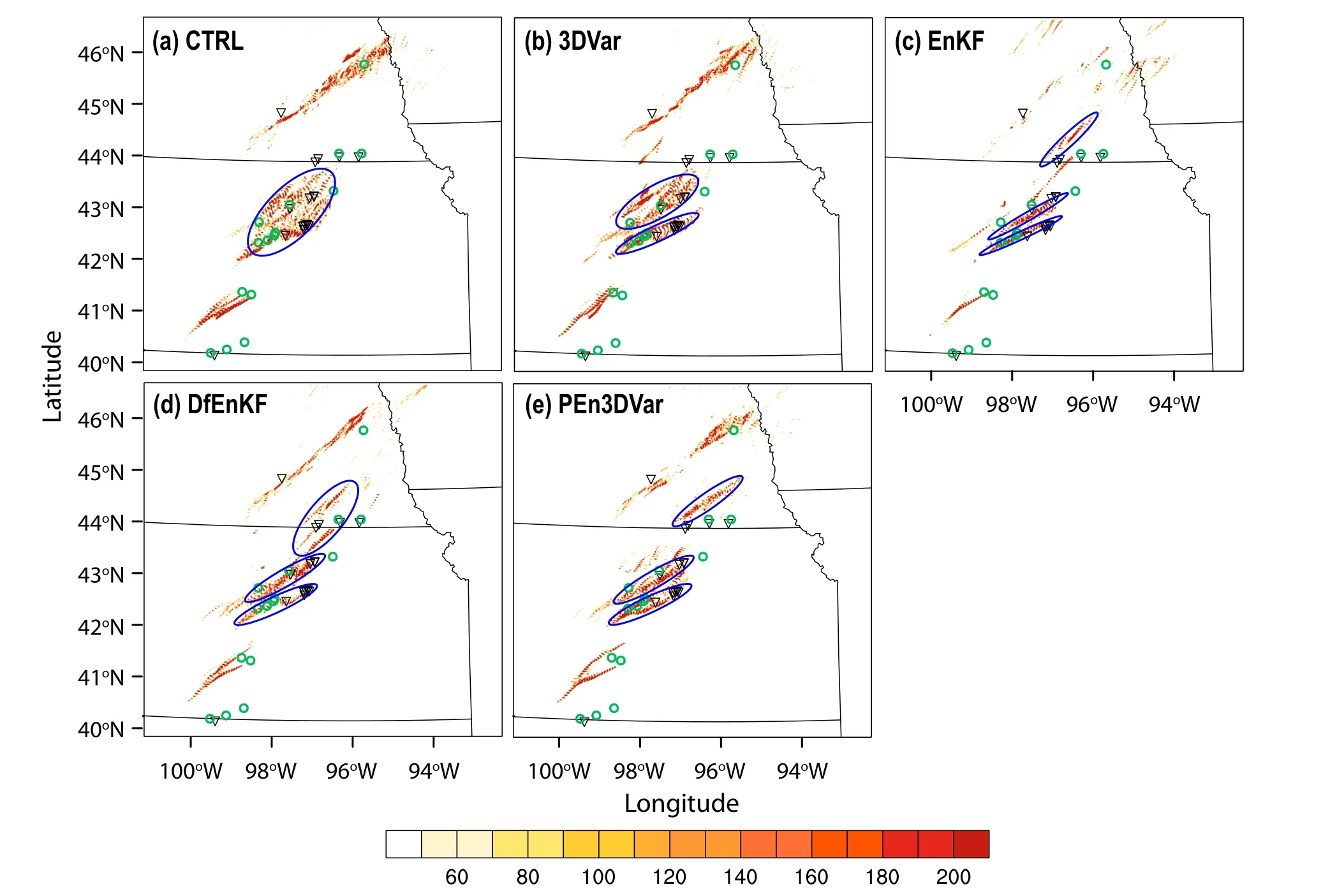
Fig.9.The 0-2-h forecast for the 2-5 km updraft helicity (m2 s-2) for the supercell case from (a) CTRL,(b) 3DVar,(c)EnKF,(d) DfEnKf,and (e) PEn3DVar,respectively,overlaid with tornado reports (inverted triangle) and hail reports (green circles) during the same time period.

5.Summary and conclusions

In this study,the capability to assimilate GOES-R GLM data within the GSI hybrid ensemble-variational(EnVar) system for convection-allowing NWP was developed.Real GOES-R GLM FED data are assimilated into a convection-resolving WRF model for a supercell storm case over the Great Plains of the United States using the hybrid En3DVar method,EnKF,as well as the DfEnKF and,3DVar methods.The FED observation operator based on graupel mass from Kong et al.(2020) is used for the assimilation.One-minute FED rates are assimilated every 5 min for a 1-h period and 4-h deterministic forecasts are produced from the final analyses of each DA method.

DA experiments using EnKF,DfEnKF,3DVar,and hybrid En3DVar are performed,and their performances are evaluated and compared against each other as well as against a control run (CTRL) that does not assimilate any data.Objective verifications employing neighborhood ETS are performed for simulated FED and reflectivity.The main findings from this evaluation are summarized as follows:

● Single-point experiments are conducted and compared between DfEnKF and pure En3DVar at uses 100%ensemble covariance (PEn3DVar).Without applying vertical localization in both En3DVar and EnKF,the magnitudes and horizontal extents of the analysis increments of the hydrometeors of graupel,snow,and rainwater for PE3DVar are much larger than EnKF.The differences in the analysis increments are mainly caused by the localization and the horizontal/vertical integration of the graupel mass in the observation operator.

● The analyses after 1-h DA and the ensuing 4-h forecasts of FED in EnKF,DfEnKF,3DVar,and PEn3DVar are compared with those of CTRL as well as GLM FED observations.All DA experiments generally capture the three discrete FED cores better than CTRL in the analyses.The high FED values in CTRL appear more linear in structure and lack discrete FED core structures as observed.

● The root-mean-square innovation (RMSI) values of FED analyses and forecasts within the 1-h DA window and the follow-up 1-4 h FED forecasts for CTRL,3DVar,EnKF,DfEnKF,and PEn3DVar are compared.Overall,pure En3DVar that uses 100% ensemble covariance has a similar performance as EnKF/DfEnKF.3DVar has a smaller RMSI than CTRL during DA but increases quickly during the 1-h forecasts after the DA.The lack of consistent updating of all state variables is believed to be the main reason.

● The 0-4 h forecasts of composite reflectivity fields from different experiments are verified against WSR-88D composite reflectivity.Overall,all DA experiments produce higher ETSs than CTRL;EnKF produces slightly higher ETSs than DfEnKF and PEn3Dvar,and both are much larger than 3DVar for the threshold of 20 dBZ.

● The 0-2 h accumulated swaths of 2-5 km UH in the supercell DA experiments are compared with SPC tornado reports.EnKF,DfEnKF,and PEn3DVar all perform similarly and outperform both CTRL and 3DVar in terms of capturing the three high UH swaths in central Kansas matching the observed tornado tracks.

In summary,the experiments that assimilate FED data using EnKF,3DVar,and En3DVar are all better at capturing the intensity and distribution of storms in the analyses and forecasts in terms of FED,reflectivity,and updraft helicity,relative to CTRL that does not assimilate FED data.Overall,PEn3DVar produces comparable results to EnKF,whereas 3DVar performs the worst among all DA methods tested.This suggests that the flow-dependent cross-variable correlations used in ensemble-based DA experiments (EnKF,En3DVar) play an important role in generating physically consistent analyses of unobserved state variables,leading to improved forecasts.

Despite encouraging results obtained thus far within the operational GSI DA framework,more systematic testing and evaluations are warranted with more cases.The current operators assumed a linear relationship between FED and graupel mass or graupel volume and the operators were originally derived based on simulation data sets.The relationship between the total flash rate and graupel mass is not necessarily linear (e.g.,Fig.5a in Allen et al.,2016),and there may be large variability in the graupel mass scaling coefficient across different convective regimes.Kong et al.(2022)recently developed a new nonlinear operator for the GLM FED observations,which can be tested and compared with the old operator using variational DA methods in future work.Furthermore,the GLM FED data would eventually need to be assimilated in conjunction with other operationally available data,such as radar and GOES-R ABI radiance data.The sensitivity of data impact on the microphysics parameterization scheme should also be investigated as it directly affects thunderstorm prediction.In addition,the new DA methods can also be implemented in Joint Effort for DA Integration (JEDI,which is an innovative,next-generation U.S.DA system) and tested with the target Rapid Refresh Forecast System (RRFS,the next-generation U.S.ensemble weather forecast system) configurations.We are hopeful that after more intensive testing,such DA capabilities can be transitioned into operations in the near future.

AcknowledgementsThis work was primarily supported by NOAA JTTI award via Grant #NA21OAR4590165,NOAA GOESR Program funding via Grant #NA16OAR4320115.Auxiliary funding was also provided by NOAA/Office of Oceanic and Atmospheric Research under NOAA-University of Oklahoma Cooperative Agreement #NA11OAR4320072,U.S.Department of Commerce.This work was further supported by the National Oceanic and Atmospheric Administration (NOAA) of the U.S.Department of Commerce via Grant #NA18NWS4680063.The DA experiments were conducted on the NSF XSEDE supercomputing facility at Texas Advanced Computing Center.Auxiliary computer resources were provided by the Oklahoma Supercomputing Center for Education and Research (OSCER) hosted at the University of Oklahoma.