Impacts of Ice-Ocean Stress on the Subpolar Southern Ocean:Role of the Ocean Surface Current

Yang WU,Zhaomin WANG,Chengyan LIU,and Liangjun YAN

1School of Information Engineering, Nanjing Xiaozhuang University, Nanjing 211171, China

2Southern Marine Science and Engineering Guangdong Laboratory (Zhuhai), Zhuhai 519082, China

3College of Oceanography, Hohai University, Nanjing 210098, China

ABSTRACT The mechanical influences involved in the interaction between the Antarctic sea ice and ocean surface current (OSC)on the subpolar Southern Ocean have been systematically investigated for the first time by conducting two simulations that include and exclude the OSC in the calculation of the ice-ocean stress (IOS),using an eddy-permitting coupled ocean-sea ice global model.By comparing the results of these two experiments,significant increases of 5%,27%,and 24%,were found in the subpolar Southern Ocean when excluding the OSC in the IOS calculation for the ocean surface stress,upwelling,and downwelling,respectively.Excluding the OSC in the IOS calculation also visibly strengthens the total mechanical energy input to the OSC by about 16%,and increases the eddy kinetic energy and mean kinetic energy by about 38% and 12%,respectively.Moreover,the response of the meridional overturning circulation in the Southern Ocean yields respective increases of about 16% and 15% for the upper and lower branches;and the subpolar gyres are also found to considerably intensify,by about 12%,11%,and 11% in the Weddell Gyre,the Ross Gyre,and the Australian-Antarctic Gyre,respectively.The strengthened ocean circulations and Ekman pumping result in a warmer sea surface temperature(SST),and hence an incremental surface heat loss.The increased sea ice drift and warm SST lead to an expansion of the sea ice area and a reduction of sea ice volume.These results emphasize the importance of OSCs in the air-sea-ice interactions on the global ocean circulations and the mass balance of Antarctic ice shelves,and this component may become more significant as the rapid change of Antarctic sea ice.

Key words: subpolar Southern Ocean,Antarctic sea ice,ice-ocean stress,air-sea-ice-ocean interaction,ocean surface current,MITgcm-ECCO2

1.Introduction

The Antarctic sea ice significantly influences the Southern Ocean circulation,the polynyas,and the Antarctic Bottom Water formation by modulating the buoyancy flux and momentum flux between the atmosphere and the subpolar Southern Ocean (Hosking et al.,2013;Abernathey et al.,2016;Haumann et al.,2016;Naveira Garabato et al.,2016;Dotto et al.,2018;Jenkins et al.,2018;Campbell et al.,2019;Wang et al.,2019b;Ma et al.,2020;Wu et al.,2017b,2020).Previous studies have focused on the role of freshwater and sea ice formation/export on the meridional overturning circulation (MOC) over the Southern Ocean (Abernathey et al.,2016;Pellichero et al.,2017),and have also concluded that the Antarctic sea ice transport drives the salinity of the Southern Ocean and its recent trends,which is among the most prominent signals of climate change in the global ocean (Haumann et al.,2016).Moreover,Antarctic sea ice also modulates the momentum transfer from the atmosphere to the subpolar Southern Ocean (Pellichero et al.,2017;Dotto et al.,2018;Naveira Garabato et al.,2019;Auger et al.,2022;Ramadhan et al.,2022).Recently,Dotto et al.(2018) and Naveira Garabato et al.(2019) emphasized the importance of sea ice in modulating the wind-stress curl and the subpolar gyres in the Southern Ocean.Additionally,Auger et al.(2022) found out that sea ice-modulated ocean surface stress (OSS) induces an offshore extension of the Antarctic slope current (ASC) from autumn to winter.In a recent observational study of the Southern Ocean by Ramadhan et al.(2022),the circumpolar maps of OSS mediated by sea-ice,around Antarctica have been studied.They found that surface geostrophic currents significantly modify the stress fields.However,it is not clear how the errors in the daily sea ice motion data affect the mean OSS;noting also that the monthly geostrophic currents were mixed with daily sea ice velocity,so it remains unclear how the monthly currents affect the daily ice-ocean stress and the OSS (Ramadhan et al.,2022).Hence,a systematic study addressing the sea ice-modulated OSS and its impact on the subpolar Southern Ocean circulation is needed.

In the sea ice-covered subpolar oceans,the OSS (τ) is generally calculated by a quadratic drag law which is a combination of ice-ocean stress (τIO) and air-ocean stress (τAO):

where ρw=1028 kg m-3and ρa=1.25 kg m-3are the seawater and air densities,respectively;α is the sea ice concentration (SIC);ui,ua,and uoare the sea ice velocity,10-m wind velocity,and the ocean surface current velocity (OSC),respectively.Following previous investigations (Cole et al.,2014;Lüpkes and Birnbaum,2005),the ice-ocean drag coefficient (Cio) and the air-ocean drag coefficient (Cao) are assumed constant due to the absence of observations,so that Cao=0.00125 and Cio=0.0055.Due to the sparseness of observations,some studies (Yang,2006,2009;Pellichero et al.,2017;Dotto et al.,2018;Naveira Garabato et al.,2019) investigated the circulations in the Arctic Ocean and the subpolar Southern Ocean using the assumption that OSC and geostrophic current can be neglected in the iceocean stress and the Ekman pumping calculations.By this assumption,these studies (Pellichero et al.,2017;Dotto et al.,2018;Naveira Garabato et al.,2019) used simplified forms of Eqs.(2) and (3) as follows:

For ease in exploring the mechanisms,the ice-ocean stress is reduced to Eq.(4) in studying the ocean circulations;and,the effects of including OSC in the calculation of ice-ocean stress on the subpolar Southern Ocean circulations have not been included in these studies (Pellichero et al.,2017;Dotto et al.,2018;Naveira Garabato et al.,2019).However,previous studies have recognized that the inclusion of OSC inτAOresults in a significant negative bias in the mechanical energy input,and hence a 10%-15% reduction in the strength of the Atlantic meridional overturning circulation and the horizontal gyre circulations (Dawe and Thompson,2006;Duhaut and Straub,2006;Hughes and Wilson,2008;Eden and Dietze,2009;Scott and Xu,2009;Zhai et al.,2012;Munday and Zhai,2015;Wu et al.,2017a).Also,the inclusion of OSC in the calculation of air-ocean heat flux can significantly improve the simulated sea surface temperature (SST) (Luo et al.,2005;Deng et al.,2009;Zhao et al.,2011;Song,2020,2021).

The influences of coupling OSC in theτIOcalculation on the Beaufort Gyre and subpolar North Atlantic have been highlighted in some studies (Martin et al.,2014;Tsamados et al.,2014;Kwok and Morison,2017;Meneghello et al.,2017,2018a,b;Dewey et al.,2018;Zhong et al.,2018;Wang et al.,2019a;Wu et al.,2021).For example,Meneghello et al.(2018a) found a fundamental mechanism,termed an “ice-ocean stress governor”,in modulating the depth,strength,and freshwater content of the Beaufort Gyre.Meanwhile,a more than 15 m yr-1decrease of Ekman pumping,is found over Beaufort Gyre when the OSC is considered inτIOin winter (Meneghello et al.,2018b).Such a negative Ekman pumping anomaly leads to a 25% decrease in the freshwater content over the Beaufort Gyre (Wang et al.,2019a).Moreover,Wu et al.(2021) found there is a visible reduction in the OSS and Ekman pumping over the subpolar North Atlantic and the Nordic Seas when the OSC is included in theτIOcalculation.This decrease further weakens the oceanic kinetic energy and visibly affects the ocean circulations (Wu et al.,2021).Ramadhan et al.(2022) found that the OSS in the subpolar Southern Ocean was significantly modulated by the surface geostrophic currents.In general,the Antarctic sea ice is thinner (order 1 m) and much more mobile and loosely packed than that in the Arctic.Hence,the OSS in the subpolar Southern Ocean is expected to be very different from that in the Arctic Ocean when OSC is considered in theτIOcalculation.A few studies have reported on the mechanical impact of the interaction between the Antarctic sea ice and OSC on the subpolar Southern Ocean(Kim et al.,2017;Ma et al.,2020).

In this study,we use two different parameterizations of ice-ocean stress (Eqs.2 and 4) to investigate the mechanical influences of the interaction between the Antarctic sea ice and the OSC on the air-sea-ice fluxes,the momentum transfer from the atmosphere to the subpolar Southern Ocean,which has not been systematically addressed in previous investigations (Pellichero et al.,2017;Dotto et al.,2018;Naveira Garabato et al.,2019;Ramadhan et al.,2022).Our study can also be considered to be an extension of Dotto et al.(2018)and Ramadhan et al.(2022) in the subpolar Southern Ocean,who assessed its circulation using satellite altimetry and computed the surface stress and stress curl acting on the gyre;however,Dotto et al.(2018) did not consider the role of the OSC and there were unknown uncertainties in the data used in Ramadhan et al.(2022).

The remainder of this paper is structured as follows.Section 2 presents the experimental designs and briefly outlines the model configuration.Section 3 describes and discusses the influence of including OSC in the τIOcalculation on the air-sea-ice fluxes,mechanical energy input,and the subpolar gyres.This paper concludes by providing a summary of the major findings and a discussion in section 4.

2.Model and Experimental setup

In this study,we employed MITgcm-ECCO2 (Menemenlis et al.,2008).The MIT general circulation model was used to develop MITgcm-ECCO2 (Marshall et al.,1997a,b)which is the state estimate configuration used in Estimating the Climate and Circulation of the Ocean Phase 2.A cubesphere grid configuration is employed in MITgcm-ECCO2 to avoid polar singularities (Adcroft et al.,2004).The mean horizontal grid size of MITgcm-ECCO2 is about 18 km (i.e.,eddy-permitting) and there are with 50 unevenly spaced vertical levels are used in this model with thicknesses increasing from 10 m near the surface to 450 m at the ocean bottom.A sea ice model (Losch et al.,2010) is coupled with the ocean model.The MITgcm-ECCO2 is run with optimized control parameters by the Green Function approach (Menemenlis et al.,2008).More details about the MITgcm-ECCO2 are available in Wu et al.(2016,2017b,2020,2021).

The Japanese 55-year Reanalysis dataset (JRA55)(Kobayashi et al.,2015) is used to force this model,including the 10-m wind,2-m air temperature,2-m specific humidity,6-hourly downward longwave and shortwave radiation,and precipitation.The MITgcm-ECCO2 has been integrated by using the forcing data from 1979 to 2018,and this experiment is defined as the CONTROL run.To examine the mechanical effects of the interaction between Antarctic sea ice and OSC on the subpolar Southern Ocean,we also conducted a sensitivity experiment (named NONE) in which the OSC was excluded in the τIOcalculation,i.e.,Eq.(4) is used in the integration of the NONE experiment.Specifically,the simple parameterization of ice-ocean stress (Eq.4) has been applied both to the ice model and ocean model;and a judgment of the ice-ocean stress direction has been made when calculating the ice-ocean stress.If ice moves faster than the current,the momentum is transferred from the ice to the current.In the opposite process,the momentum is transferred from the current to the ice.Therefore,the differences in the simulated results between CONTROL and NONE are the result of the difference between Eqs.(2) and (4),thereby reflecting the mechanical influences of the interaction between the sea ice and OSC on the subpolar Southern Ocean.These two experiments are both integrated from 1979 to 2018 and initialized with the same climatology.Monthly averaged model outputs at 18-km resolution for the last 10 years (2009-2018) are used here.

3.Results

3.1.Air-sea-ice fluxes

Figure 1a shows the time-mean zonal OSS in CONTROL.Similar to previous results (Wu et al.,2016,2020)and zonal OSS in NONE (not shown),the spatial distribution of zonal OSS is featured by broad large values in the Antarctic Circumpolar Current (ACC) area,and small values in the regions covered by sea ice (within the black line),by relatively large values in the Antarctica coastal regions and near the sea ice edge.When the OSC is excluded in the τIOcalculation,there is a broad increase in the westward OSS at higher latitudes,especially close to the Antarctica coastal regions,and in the eastward OSS at lower latitudes,most notably near the sea ice edge (Fig.1b).Such a pattern is more pronounced for the winter period (July-August-September)than for the whole year (Fig.1c).For the meridional component,the spatial pattern is featured by positive values in the Weddell Sea (WS;60°-80°S,40°W-0°),the Ross Sea (RS;60°-80°S,130°W-175°E),and the Antarctica coastal regions,especially between 45° and 180°E,and large negative values in the broad ACC region (Fig.1d).A broad and significant increase in the northward component is found,while a large increase in the southward component is found in the coastal region when the OSC is excluded in the ice-ocean stress calculation (Fig.1e).Such a pattern is also more pronounced in winter (Fig.1f).These changes are induced by the exclusion of the northward and southward OSC in these regions (not shown).

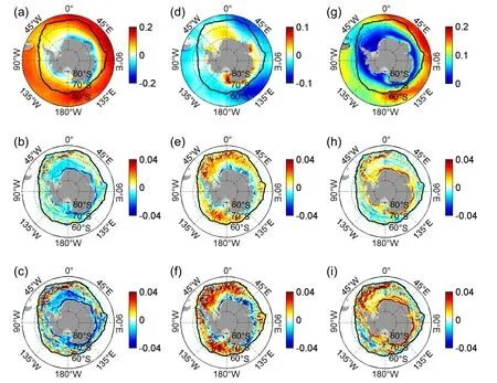
Fig.1.(a) The time-mean zonal ocean surface stress (N m-2) in CONTROL.(b) The differences in the time-mean zonal ocean surface stress between CONTROL and NONE (NONE minus CONTROL).(c) Same as in (b),but for the winter mean(from July to September).Panels (d)-(f) and (g)-(i) are similar to (a)-(c),but for the meridional ocean surface stress (N m-2)and the magnitude of the ocean surface stress (N m-2),respectively.Black lines in this figure (and the following figures)denote the annual and winter 15% sea ice concentration averaged over the last decade in CONTROL.

Similar to the pattern of zonal OSS,the spatial distribution of the magnitude of the OSS features large values in the ACC area and the Antarctica coastal regions,and small values in the regions covered by sea ice (Fig.1g).The magnitude of the time-mean OSS significantly increases in the annual mean OSS,especially in the WS,RS,and the Antarctica coastal regions (Figs.1h,i).Averaged over areas to the south of 60°S,the magnitude of the time-mean OSS is about 5% stronger in NONE than that in CONTROL,while an increase of about 20% is found in the WS region (Table 1).In winter,increases of about 8% and 27% are found over and to the south of 60°S and in the WS,respectively,from CONTROL to NONE (Table 1).The significant increase of the OSS in the Antarctica coastal regions indicates that the OSCs are generally orientated in the direction of the sea ice drift (Figs.1b,c).

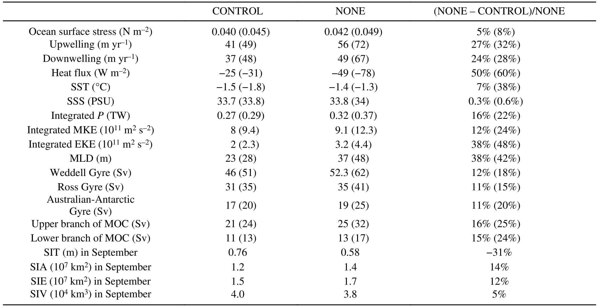
Table 1.Diagnostics from the CONTROL and the NONE over the south of 60°S.The percentage of the differences to the NONE between the CONTROL and the NONE are also given.Values in the bracket are corresponding to the values averaged over the winter mean (July-August-September).

The map of the annual mean Ekman pumping is presented in Fig.2a.Large-scale upwelling and downwelling are found in the region covered by sea ice,especially around east Antarctica.The exclusion of OSC in the ice-ocean stress calculation leads to substantially enhanced upwelling and downwelling in the higher latitudes of the sea-ice-covered region,especially around east Antarctica (Figs.2b,c).There are some scattered negative values in Figs.2b and 2c,especially in the marginal region of the northeastern Ross Sea (0°-45°W,50°-60°S),which are induced by the increased meridional gradient of the zonal OSS.Overall,the strength of the annual upwelling (downwelling) averaged over and to the south of 60°S is about 27% (24%) stronger in NONE than that in CONTROL,this differential response is greater in the winter mean when about a 32% (28%)increase upwelling (downwelling) is found.

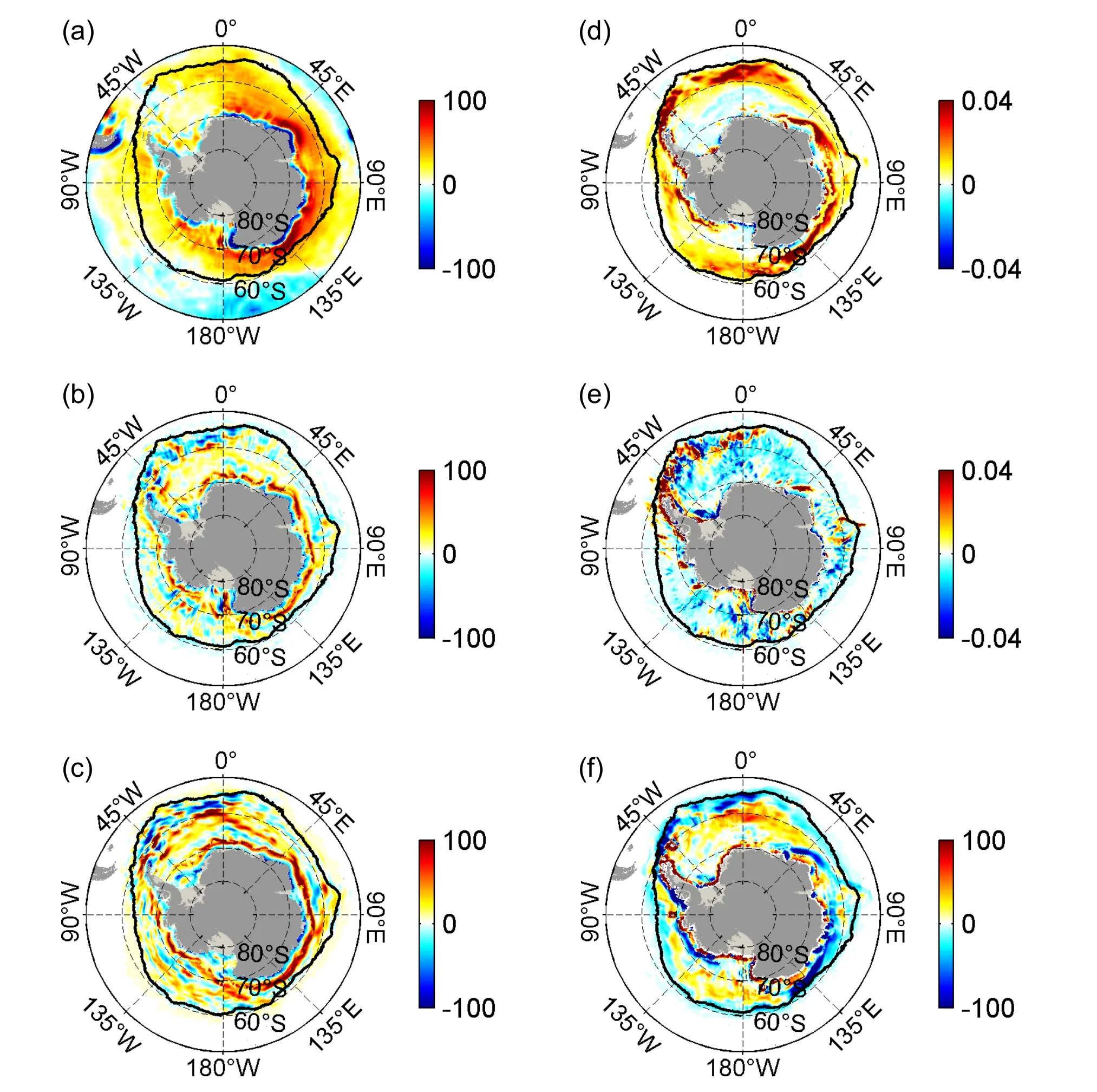
Fig.2.(a) The time-mean Ekman pumping (m yr-1) in CONTROL.(b) The differences in the time-mean Ekman pumping between CONTROL and NONE (NONE minus CONTROL).(c) Same as in (b),but for the winter mean.Panels (d) and (e) represent the difference of zonal and meridional ocean surface stresses calculated with and without the ocean ageostrophic currents in the ice-ocean stress calculation using the outputs from CONTROL (results without ageostrophic current minus results with ageostrophic current).(f) The difference between Ekman pumping calculated with and without the ocean ageostrophic currents using the outputs from CONTROL (result without ageostrophic currents minus result with ageostrophic currents).The Ekman pumping and ocean surface stress fields have been smoothed using a 4-point box filter.

Due to the scarcity of observations,the surface geostrophic current was often used in previous investigations to replace the total OSC (ageostrophic and geostrophic components) when calculating Ekman pumping in the sea-ice-covered region (Zhong et al.,2018).In this study,the different results that arise from including only the surface geostrophic current as opposed to including the total OSC in the Ekman pumping and ice-ocean stress calculations have also been studied (Figs.2d-f).Weakening the total OSC to the surface geostrophic current significantly reduces the zonal and meridional OSS,especially in the WS,the RS,and the Antarctica coastal regions (Figs.2d,e).The distribution and magnitude of OSS diagnosed by only using the surface geostrophic current significantly differ from those calculated by using both the ageostrophic and geostrophic components,especially in the WS,the RS,while close to Antarctica,the difference virtually disappears (Figs.2d,e).Significant differences in the pattern and the magnitude are also found for the Ekman pumping (Fig.2f).The above results present that the surface ageostrophic current plays an important role in the ice-ocean stress calculation and the Ekman pumping.In future investigations,the surface ageostrophic current should be considered properly rather than only considering the surface geostrophic current when calculating the ice-ocean stress.

Figure 3 shows the spatial pattern of the net ocean surface heat flux in CONTROL,and the differences between these two simulations for the annual mean and winter mean.The spatial distributions of the net ocean surface heat flux in CONTROL are very similar to those in NONE,featuring the loss of heat (negative values) in the sea-ice-covered subpolar regions (Fig.3a).When excluding OSC in the iceocean stress calculation,enhanced heat loss occurs in the subpolar Southern Ocean,especially in the WS,the RS,and broad regions around East Antarctica (Fig.3b).These differences are much more pronounced in winter compared to those in the annual mean (Fig.3c).Overall,heat loss averaged over the subpolar Southern Ocean (south of 60°S) decreases by about 50% from NONE (49 W m-2) to CONTROL(25 W m-2) (Table 1).For the winter,the heat loss decreases by about 60% averaged over the south of 60°S from NONE (78 W m-2) to CONTROL (31 W m-2;Table 1).

Fig.3.(a) The time-mean net heat flux (W m-2) in CONTROL.The positive values denote heat gain from the atmosphere to the ocean,and the negative values denote heat loss from the ocean to the atmosphere.(b) The differences in annual mean net heat flux between CONTROL and NONE (NONE minus CONTROL).(c) Same as in (b),but for the winter mean.

Differences in the surface heat loss in the subpolar Southern Ocean between CONTROL and NONE are associated with the SST and SIC differences induced by excluding the OSC in the ice-ocean stress calculation (Fig.4).The differences in the strengths of Ekman Pumping are in part responsible for the differences of SST between CONTROL and NONE in the subpolar Southern Ocean (Fig.2).In addition to the warming effect of the enhanced Ekman pumping,the broad reduction of SIC in NONE is also caused by the stronger ice-ocean stress in NONE than that in CONTROL(Fig.1).The reduction of SIC,along with the surface warming,leads to increased heat loss from CONTROL to NONE.In NONE,the strengthened Ekman pumping also leads to a broad increase in sea surface salinity (SSS,Fig.4e),particularly in the winter (Fig.4f).There is a significant SSS anomaly in the eastern Weddell Sea (Figs.4e,f) which is induced by the salinity accumulation from the increased Antarctic slope current as shown below.The above results demonstrate that the differences in the ocean surface heat flux between CONTROL and NONE over the subpolar Southern Ocean are dominated by the indirect effects of considering OSC in the ice-ocean stress calculation.Note that all the differences between the two experiments are significant at the 95% level,based on a Student’st-test.

Fig.4.(a) The time-mean SST (oC) in CONTROL.(b) The difference of time-mean SST between CONTROL and NONE (NONE minus CONTROL).(c) Same as in (b),but for the winter mean.(d)-(f) Same as in (a)-(c),but for the SSS (PSU).

3.2.Mechanical Energy Input and Kinetic Energy

The total mechanical energy input (P) is diagnosed as,where the overbar represents the last 10-year time mean;τand u are the OSS and OSC,respectively.The distributions ofPin these two simulations are similar to the previous investigations (Huang et al.,2006;von Storch et al.,2012;Zhai et al.,2012;Wu et al.,2016,2020),with large values concentrated in the broad ACC area and the Antarctic continental slope (Fig.5a).Figure 5b shows that the increase inPfrom CONTROL to NONE is significant in the WS,RS,and Antarctic continental slope.This is especially true in winter when there is a much more pronounced increase (Fig.5c).A similar result is also found for the wind power input to the time-varying velocity by the time-varying OSS (,Figs.5d-f),where the prime represents the deviation from the last 10-year mean.Spatially integratedPover and to the south of 60°S is 0.32 TW (1 TW=1012W) in NONE;about 0.21 TW and 0.11 TW are corresponding to the time-mean part (·) and the time-varying part (),respectively.In contrast,the integratedPin the CONTROL is only 0.27 TW;about 0.18 TW and 0.09 TW result from,respectively,representing a respective 16%,17%,and 18% reduction relative to NONE inP,,and·,respectively.Therefore,the exclusion of the OSC in the calculation of ice-ocean stress leads to a broad increase in the mechanical energy input from CONTROL to NONE.

Fig.5.(a) The time-mean mechanical energy input by time-mean ocean surface stress (W m-2) in CONTROL.(b)The difference of time-mean mechanical energy input between CONTROL and NONE (NONE minus CONTROL).(c) Same as in (b),but for the winter mean.(d)-(f) Same as in (a)-(c),but for time-varying mechanical energy input by time-varying ocean surface stress (W m-2).

The spatial pattern of the surface eddy kinetic energy(EKE) and mean kinetic energy (MKE) are given in Fig.6,and their differences between CONTROL and NONE are also given.Here,the EKE is defined as,where v and u are meridional and zonal velocities.The distribution of EKE is featured by large patchy values in the broad Southern Ocean and small values in the sea-ice-covered region(Fig.6a).Such a spatial pattern suggests that the sea ice can suppress the eddy activities in the subpolar Southern Ocean.Consistent with the previous study (Wu et al.,2021),excluding OSC in the ice-ocean stress calculation leads to a widespread incremental increase in the surface EKE(Figs.6b,c).The EKE increase is most pronounced in the WS and the RS (Figs.6b,c).In comparison,the spatial pattern of CONTROL is almost the same as that in NONE,confirming that the decrease of the EKE is mainly caused by the relative ice-ocean surface current effect (Figs.6a-c).Spatially integrated over the areas covered by sea ice,the EKEs are 3.2×1011m2s-2and 2×1011m2s-2in the NONE and the CONTROL,respectively,representing a reduction of 38%from NONE to CONTROL (Table 1).The surface EKEs integrated over the WS and the RS in CONTROL are 63% and 71% less than those in NONE,respectively.The EKE increase is much more pronounced in the winter,amounting to a 48% increase when integrated over and to the south of 60°S (Fig.6c).It is also found that the increase of EKE is visible at the sea surface,with a gradual decrease to 400 m and a sharp decrease below 400 m (not shown).

Fig.6.(a) The time-mean EKE (m2 s-2) in CONTROL.(b) The difference of time-mean EKE between CONTROL and NONE (NONE minus CONTROL).(c) Same as in (b),but for the winter mean.(d)-(f) Same as in (a)-(c),but for MKE (m2 s-2).

Similarly,the pattern of MKE is also depicted by large values in the broad Southern Ocean,the Antarctic continental slope,and small values in the sea-ice-covered region(Fig.6d).Excluding the OSC in the ice-ocean stress calculation leads to an incremental increase of the surface MKE over most of the subpolar Southern Ocean,most significantly around Antarctica,i.e.,in the WS,RS,and Prydz Bay(Fig.6e).This increase is also significant in the winter(Fig.6f).For example,integrated over the oceans with sea ice coverage,the MKE decreases by about 12% from 9.1 ×1011m2s-2in NONE to 8×1011m2s-2in CONTROL(Table 1).In contrast to the vertical distribution of the EKE increment,the MKE increment is confined within the upper 100 m (not shown).

3.3.Antarctic Sea Ice

The variability in the air-sea-ice fluxes and their consequences induced by the strengthened ice-ocean stress and Ekman pumping in NONE can feedback to the sea ice.As shown in Fig.7,the SIC weakens broadly in NONE,particularly in the WS,RS,and Prydz Bay,as a combination of the strengthened sea ice drift and higher SST that occurs when the sea ice drift is decoupled from the OSC in NONE(Figs.7b,c).Overall,the annual mean SICs are 48% and 45%in CONTROL and NONE,respectively,representing a 6%reduction relative to CONTROL.In winter,the SICs are 61%and 54% in CONTROL and NONE,representing an 11%reduction relative to CONTROL.Figure 7d shows the timemean distribution of sea ice thickness (SIT),characterized by large SIT in the WS and RS as well as sea ice drift vectors,which show large drifts in the sea ice marginal zone and the Antarctic slope area.Similarly,the annual mean SIT decreases by 31%,from 0.76 m in CONTROL to 0.58 m in NONE (Fig.7e);in the winter,this reduction amounts to 28%(0.81 m in CONTROL and 0.58 m in NONE) (Fig.7f).In NONE,the OSC is much stronger than that in CONTROL,and the sea ice drift is strengthened by the weaker ice-ocean stress felt by sea ice in NONE than that in CONTROL,especially in the marginal areas of sea ice and along the Antarctic slope region (Fig.7e).This strengthened sea ice drift also becomes much more pronounced in the winter mean results(Fig.7f).

Fig.7.(a) Distributions of the time-mean sea ice concentration (%) in CONTROL.(b) The difference of time-mean sea ice concentration between CONTROL and NONE (NONE minus CONTROL).(c) Same as in (b),but for the winter mean.(d)-(f) Same as in (a)-(c),but for sea ice thickness (m),the vectors denote the corresponding sea ice drift (m s-1).

Figure 8 presents the climatology of the monthly mean total Antarctic sea ice volume (SIV),sea ice extent (SIE),and sea ice area (SIA).The total SIA and the SIE are much larger,while the total SIV is smaller,in NONE than those in CONTROL.For example,the SIA in September increases from about 1.2×107km2in CONTROL to about 1.4 ×107km2in NONE.Similarly,the SIE in September increases from about 1.5×107km2in CONTROL to about 1.7×107km2in NONE (Table 1).In contrast,the total SIV in September decreases from 4.0×104km3in CONTROL to 3.8×104km3in NONE (Fig.8c).The significant increases in the total SIA and the SIE in NONE are attributed to the strengthened sea ice transport caused by the weak ice-ocean stress felt by sea ice,as shown above(Figs.7e,f).The reduced total SIV is induced by the thinner SIT (Figs.7e,f),presumably caused by the warmer SST(Figs.4b,c) and larger sea ice drift (Figs.7d-f) in NONE compared to those in CONTROL,as analyzed above.

Fig.8.Simulated monthly (a) total Antarctic SIA (km2),(b)total SIE (km2),and (c) the SIV (km3) in the CONTROL(black solid line) and NONE (black dashed line) simulations.

3.4.Subpolar Gyres and Meridional Overturning Circulation

The increases in the OSS and mechanical energy input in NONE intensify the subpolar gyres and OSC (Fig.9).It can be seen that the OSC broadly increases in the subpolar gyres,especially in the WG,RG,and the Antarctic slope current region (Fig.9b).Consistent with their larger annual increases,the OSC increases are much more pronounced in winter (Fig.9c).The changes in the barotropic stream function indicate the strengthening of the subpolar gyres in NONE (Figs.9b,c).Quantitatively,the WG weakens by about 12% from NONE (52.3 Sv) to CONTROL (46 Sv),and the RG slows down by 11% from NONE (35 Sv) to CONTROL (31 Sv).Also,an 11% weakening of the Australian-Antarctic Gyre (AAG) is found between NONE (19 Sv) and CONTROL (17 Sv).Following Wang and Meredith (2008),the strength of the AAG,RG,and WG are calculated as the maximum of the barotropic stream function at 110°E,150°W,and the Prime Meridian,respectively.These reductions are much more pronounced in winter,amounting to about 18%,15%,and 20% for the WG,RG,and AAG,respectively (Table 1).

Fig.9.(a) Distributions of the time-mean barotropic stream functions (Sv) in CONTROL.(b) The difference of time-mean barotropic stream functions between CONTROL and NONE(NONE minus CONTROL).(c) Same as in (b),but for the winter mean.The vectors represent the corresponding ocean surface currents.

We analyzed the impacts of including the OSC on the mixed layer depth (MLD) over the subpolar Southern Ocean.The definition of the MLD is the depth where the potential density is 0.03 kg m-3larger than that at the surface(Liu et al.,2017;Wu et al.,2020).The spatial patterns of the MLD and the changes between these two experiments are also shown in Figs.10a-c.The distributions of the MLD in these two simulations are characterized by a shallow MLD over the regions covered by sea ice and a deep MLD in the areas north of the ACC (Fig.10a),similar to the previous observations and simulated results (Wu et al.,2016,2020;Pellichero et al.,2017;Wilson et al.,2019).When excluding the OSC in the ice-ocean stress calculation,the MLD enlarges considerably in high latitudes,especially in the WS,RS,and Antarctic continental slope (Fig.10b).Such as,the time-mean MLD averaged over the WS in NONE and CONTROL is 37 and 23 m respectively,representing a 38% decrease.As shown in Fig.2,the increased Ekman pumping (i.e.,wind stress curl) leads to strengthened vertical mixing in NONE,contributing to the larger SSS and hence the deeper MLD in the subpolar Southern Ocean than that in CONTROL.

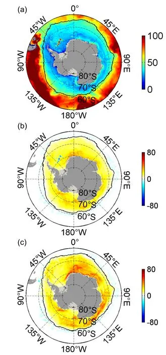
Fig.10.(a) Distributions of the time-mean MLD (m) in CONTROL.(b) The difference of MLD between CONTROL and NONE (NONE minus CONTROL).(c) Same as in (b),but for the winter mean.

Any processes that can affect the OSS and sea ice drift have an important effect on MOC in the Southern Ocean.Hence,the differences in the OSS and sea ice between these two simulations are expected to have a significant influence on the MOC in the Southern Ocean (Eden and Willebrand,2001;Zhai et al.,2014;Wu et al.,2016).The MOC in the Southern Ocean is defined by zonally integrating over the Southern Ocean from its southern boundary (xS) to the northern bounda∫ry (∫ xN),and from the bottom at z=-h upward:(x,y,z,t)dxdz(Wu et al.,2020).Figure 11a shows the structure of the MOC in the Southern Ocean,featured by the clockwise upper and counter-clockwise lower branches (Fig.11a).When excluding the OSC in the calculation of the ice-ocean stress,there are increases in the strength of the upper and lower branches of the MOC.The strength of the upper branch of the MOC weakens by about 16% from NONE (25 Sv) to CONTROL (21 Sv).There is also a decrease of 15% in the strength of the lower branch in the abyssal ocean from 13 Sv in NONE to 11 Sv in CONTROL.More intensification can be found in the winter,with the upper and lower branches increasing by about 8 Sv and 4 Sv,respectively (Fig.11c).

As shown in Figs.1 and 2,a significant increase in the OSS and Ekman pumping is concentrated along the Antarctic continental slope.As expected,the effects of excluding the OSC lead to a remarkable response in the Antarctic slope current in NONE (Fig.12).Figure 12 gives the vertical structures of the zonal velocity at the sections of 0° and 150°W across the center of the WG and RG,respectively.The Antarctic slope current substantially strengthens in NONE (Figs.12b,e),especially in the winter (Figs.12c,f).The zonal velocity in the Antarctic slope current increases by about 79% and 71% at 0° and 150°W,respectively,in the annual mean;noting that the increases are nearly double in the winter.The inclusion of the OSC in the calculation of the ice-ocean stress can thus lead to a profound influence on the global ocean circulations and the mass balance of Antarctic ice shelves,by influencing the MOC in the Southern Ocean and the Antarctic slope current.

Fig.12.(a) The time-mean vertical structure of zonal velocity (m s-1) across the Prime Meridian in CONTROL.(b)The difference in the vertical structure of zonal velocity between CONTROL and NONE (NONE minus CONTROL).(c) Same as in (b),but for the winter mean.(d)-(f) Same as in (a)-(c),but for the zonal velocity across 150°W.The negative values represent the westward Antarctic Slope Current,while the positive values represent the eastward Antarctic Circumpolar Current.

4.Conclusion and Discussion

In this study,we have studied the impacts of including the OSC in the ice-ocean stress calculation on the surface air-sea-ice flux and oceanic circulations over the subpolar Southern Ocean using a coupled ocean-sea ice global model with an eddy-permitting resolution for the first time.By comparing the model results that exclude and include OSC in the calculation of the ice-ocean stress,we have arrived at the following conclusions.

• The exclusion of the OSC in the calculation of the iceocean stress leads to an incremental increase in the magnitude of the time-mean OSS (upwelling and downwelling) by about 5% (27% and 24%),amounting to a 50% increase in the surface net heat loss,especially in the WS and the RS.This increase in the surface net heat loss is closely linked with the warm SST and the decrease in SIC.

• Excluding the OSC in the calculation of the ice-ocean stress enlarges the total wind power input to the OSC by 0.05 TW,corresponding to an increase of 16% relative to the result in the experiment that includes the OSC.This increment of the mechanical energy input leads to an increase of about 38% and 12% in the EKE and MKE integrated over the subpolar Southern Ocean,respectively.

• The increased OSS and mechanical energy input when excluding the OSC in the calculation of the ice-ocean stress lead to the intensifications of the WG,RG,and AAG,by 12%,11%,and 11%,respectively.Also,the upper and lower branches of the MOC in the Southern Ocean are intensified by about 16% and 15%.In addition,the Antarctic slope current also significantly intensifies,with the current increasing by 79% and 71% at 0° and 150°W,respectively.

Results from our study show that the resultant iceocean interactions attained by coupling the OSC in the iceocean stress calculation lead to visible influences on the air-sea-ice fluxes and the strength of the simulated oceanic general circulations on long timescales in the subpolar Southern Ocean.This study quantifies the effects of this interaction on the subpolar Southern Ocean and its feedback on the Antarctic sea ice.The consideration of the relative motion of sea ice velocity and OSC in the ice-ocean stress calculation is an integral part of the ice-ocean interaction (Ma et al.,2020);previous studies that do not consider this process are too strongly driven and lack a pivotal energy sink (Pellichero et al.,2017;Dotto et al.,2018;Naveira Garabato et al.,2019).The ice-ocean interaction coupling from the OSC should be fully considered in future studies.Meanwhile,our study also suggests a direction for improving the accuracy of sea ice simulation in the future.

It is worth emphasizing that this study expands and complements the previous investigation that focuses on the North Atlantic Ocean (Wu et al.,2021),in addition to the investigations which concern the momentum transfer from the atmosphere to the subpolar Southern Ocean (Pellichero et al.,2017;Dotto et al.,2018;Naveira Garabato et al.,2019;Auger et al.,2022;Ramadhan et al.,2022).Compared to the Arctic sea ice,Antarctic sea ice is loosely packed,relatively thin (order 1 m),and more mobile.Hence,the influences of ice-ocean interactions on the subpolar Southern Ocean are expected to be more significant when the OSC is coupled in the ice-ocean stress calculation.In addition to the quantified results,we also conducted some unique research that is distinct from Wu et al.(2021).For example,this study focused on the large-scale effects over the entire subpolar Southern Ocean rather than the relatively smaller domain of the North Atlantic Ocean.The spatial distributions of the OSS and the Ekman pumping mediated by the Antarctic sea ice over the subpolar Southern Ocean have been studied systematically;therefore our study complements the recent investigations that are based on the sparse observations (Auger et al.,2022;Ramadhan et al.,2022).In addition,the effects of the ice-ocean-interaction coupling from the OSC on the temperature and salinity over the subpolar Southern Ocean are also studied in detail which was not done in Wu et al.(2021).Meanwhile,the feedback of this ice-ocean interaction on the Antarctic sea ice and slope currents in this study are also investigated for the first time.Given the importance of the subpolar Southern Ocean in the global climate system(Abernathey et al.,2016;Haumann et al.,2016;Jenkins et al.,2018;Campbell et al.,2019) and the significant influences of coupling OSC in the air-sea-ice fluxes (Wu et al.,2017a,2021),it is necessary to visit the role of this process on the subpolar Southern Ocean in this study.There are still several limitations in our study;for example,the MITgcm-ECCO2 used in this study was conducted with only an eddypermitting resolution;and the model results are deficient,especially in high latitudes.Hence,the effects of relative ice velocity to the OSC on the subpolar Southern Ocean circulations are also deficient.Also,the forcing is too coarse to resolve the small-scale atmospheric activities which are important for the sea ice drift (Wu et al.,2016,2020).Despite these above limitations,some results presented here may quantitatively depend on the numerical model employed.The potentially significant influence of coupling the OSC in the bulk formulas that govern ocean circulation,sea ice,and climate requires future research.

Acknowledgements.This study was supported by the Independent Research Foundation of Southern Marine Science and Engineering Guangdong Laboratory (Zhuhai) (Grant No.SML2021SP306),National Natural Science Foundation of China (Grant Nos.41941007,41806216,41876220,and 62177028),Natural Science Foundation of Jiangsu Province (Grant No.BK20211015),China Postdoctoral Science Foundation (Grant Nos.2019T120379 and 2018M630499),and by the Talent start-up fund of Nanjing Xiaozhuang University (Grant No.4172111).The atmospheric forcing data were obtained freely from the NCAR’s research data archive (JRA-55: https://rda.ucar.edu/datasets/ds625.0/).The model results presented in this article are available from the authors on request.We thank the anonymous reviewers for their helpful comments that led to an improved manuscript.