Real-time arrival picking of rock microfracture signals based on convolutional-recurrent neural network and its engineering application
Bing-Rui Chen,Xu Wang*,Xinhao Zhu,Qing Wang,Houlin Xie
a State Key Laboratory of Geomechanics and Geotechnical Engineering,Institute of Rock and Soil Mechanics,Chinese Academy of Sciences, Wuhan,430071,China
b University of Chinese Academy of Sciences, Beijing,100049, China
Keywords: Rock mass failure Microseismic event P-wave arrival S-wave arrival Deep learning
ABSTRACT Accurately picking P-and S-wave arrivals of microseismic (MS) signals in real-time directly influences the early warning of rock mass failure.A common contradiction between accuracy and computation exists in the current arrival picking methods.Thus,a real-time arrival picking method of MS signals is constructed based on a convolutional-recurrent neural network (CRNN).This method fully utilizes the advantages of convolutional layers and gated recurrent units (GRU) in extracting short-and long-term features,in order to create a precise and lightweight arrival picking structure.Then,the synthetic signals with field noises are used to evaluate the hyperparameters of the CRNN model and obtain an optimal CRNN model.The actual operation on various devices indicates that compared with the U-Net method,the CRNN method achieves faster arrival picking with less performance consumption.An application of large underground caverns in the Yebatan hydropower station (YBT) project shows that compared with the short-term average/long-term average (STA/LTA),Akaike information criterion (AIC)and U-Net methods,the CRNN method has the highest accuracy within four sampling points,which is 87.44%for P-wave and 91.29%for S-wave,respectively.The sum of mean absolute errors(MAESUM)of the CRNN method is 4.22 sampling points,which is lower than that of the other methods.Among the four methods,the MS sources location calculated based on the CRNN method shows the best consistency with the actual failure,which occurs at the junction of the shaft and the second gallery.Thus,the proposed method can pick up P-and S-arrival accurately and rapidly,providing a reference for rock failure analysis and evaluation in engineering applications.
1.Introduction
Microseismic (MS) monitoring is an effective monitoring and early warning technology for rock mass failure (Cook,1976;Zhao et al.,2022;Li et al.,2023b),which has been widely used in deep rock engineering (Young and Collins,2001;Durrheim et al.,2005;Feng et al.,2019;Li et al.,2023a;Mao et al.,2023).MS monitoring analyzes the spatiotemporal evolution mechanism of rock microfractures and achieves rock failure prediction through waveform recognition,arrival picking,source positioning,and source parameter inversion in sequence (Xiao et al.,2016;Zhang et al.,2021a).Currently,the manual processing of MS data is usually considered to have the highest accuracy and the drawbacks of high cost and latency,and the automatic processing still has a certain gap in accuracy compared to manual processing.The MS P-and Sarrivals are the calculation bases of source positioning and source parameter inversion,and the deviation of the arrivals will be quickly amplified by these subsequent steps (Akram and Eaton,2016).Thus,the accuracy and efficiency of MS arrival picking have a direct impact on the effect of rock failure monitoring.For this,various arrival-picking methods for MS P-and S-waves have been proposed,which are generally divided into traditional and machine learning methods.
The traditional methods mainly include the short-term average/long-term average(STA/LTA)method(Allen,1978,1982),the Akaike information criterion (AIC) method (Maeda,1985;Li et al.,2017),the phase arrival identification-skewness/kurtosis (PAI-S/K)method (Saragiotis et al.,2002;Nippress et al.,2010) and their variants.The STA/LTA method is widely used in practical MS monitoring due to its simplicity and rapidity.However,it has the following weaknesses: relatively low accuracy,instability due to dependence on the window length (Akram and Eaton,2016) and insensitivity to signals with a low signal-to-noise ratio (SNR).The AIC and PAI-S/K methods achieve high-accuracy arrival-picking based on changes in information or statistics.However,these methods also perform poorly on low-SNR signals (Dong et al.,2018).
Machine learning methods mainly include clustering(Zhu et al.,2016,2022;Ma et al.,2018;Guo et al.,2021;Lan et al.,2022) and deep learning methods for MS arrival picking.Deep learning methods are able to pick P-and S-arrivals simultaneously by extracting hidden features from the original MS signals.Thus,these methods are a popular focus of research because of their strong robustness and high accuracy.A few approaches use the regression method to determine the arrival sampling point directly.For example,Ross et al.(2018) used a convolutional neural network(CNN) to find the regression between waveforms and arrivals.A convolutional network named Cospy uses a two-stage structure,consisting of rough positioning followed by precise regression(Pardo et al.,2019).
In most deep learning methods,arrival picking is converted into a classification task for each sampling point,mainly using U-Net or long short-term memory(LSTM)as the backbone.The U-Net model(Ronneberger et al.,2015) is a typical encoder-decoder structure.Zhang et al.(2021b) proposed a control model for S-arrival based on the outputs of U-Net,which can be used to improve the early warning effect for rockburst.Moreover,data augmentation methods were also used for U-Net training (Zhang and Sheng,2020;Zhang et al.,2021c).The LSTM model (Hochreiter and Schmidhuber,1997) is a representative form of recurrent neural network (RNN),and is naturally suited for processing time series.Zheng et al.(2018) established a stacked model consisting of 7 LSTM layers with 1024 hidden units,which shows high accuracy for acoustic emission waveforms but implies an enormous model scale.EQTransformer (Mousavi et al.,2020) can simultaneously realize high-accuracy seismic signal detection and arrival picking.This model combines 1D (one-dimensional) convolution,residual connections,bidirectional LSTM and attention mechanism,implying a very deep encoder.Such large-scale computations may lead to performance bottlenecks when attempting to process MS signals with a high sampling frequency in real-time.Subsequently,LEQNet(Lim et al.,2022),optimized from EQTransformer and reduced the scale of the model at the cost of a slight decline in accuracy.Xu et al.(2022)used multi-channel singular spectrum analysis(MSSA) and short-time Fourier transform (STFT) to extract features from MS signals,and then input these features into the arrival-picking model containing 34 LSTM cells with 600 hidden units.It has been proven to have good accuracy,while many recursive calculations limit its application in real-time processing.In summary,high accuracy and large-scale computations are the typical characteristics of the existing deep learning methods,making these methods applicable only for post-processing.The existing methods generally have a contradiction between accuracy and computation,as shown in Fig.1.Thus,an arrival picking method with both high accuracy and low computations is of great significance for realizing real-time arrival picking and early warning of rock mass fracture.
2.Method
MS signals are the typical time series superposed by rock mass microfracture signals and environmental noise,implying changes in waveform characteristics such as frequency and amplitude.To better determine the arrivals of P-and S-waves,it is necessary to reasonably express both the short-term features (STF) and longterm features (LTF) of MS signals,which describe the instantaneous changes on the local scale and the macroscopic trend on the global scale,respectively.Thus,we first introduced the structure of the convolutional-recurrent neural network (CRNN),which is constructed from the perspective of STF and LTF extraction.Then,two targeted optimizations are introduced to ensure applicability to MS signals.Subsequently,we established a complete real-time arrival picking method based on CRNN.
2.1.CRNN model
The proposed CRNN model consists of an input layer,hidden layers,and an output layer,which are responsible for accepting rock mass microfracture signals as input,extracting the features of Pand S-arrivals,and enabling the expression and evaluation of P-and S-arrivals,respectively.The structure of the CRNN model is shown in Fig.2.
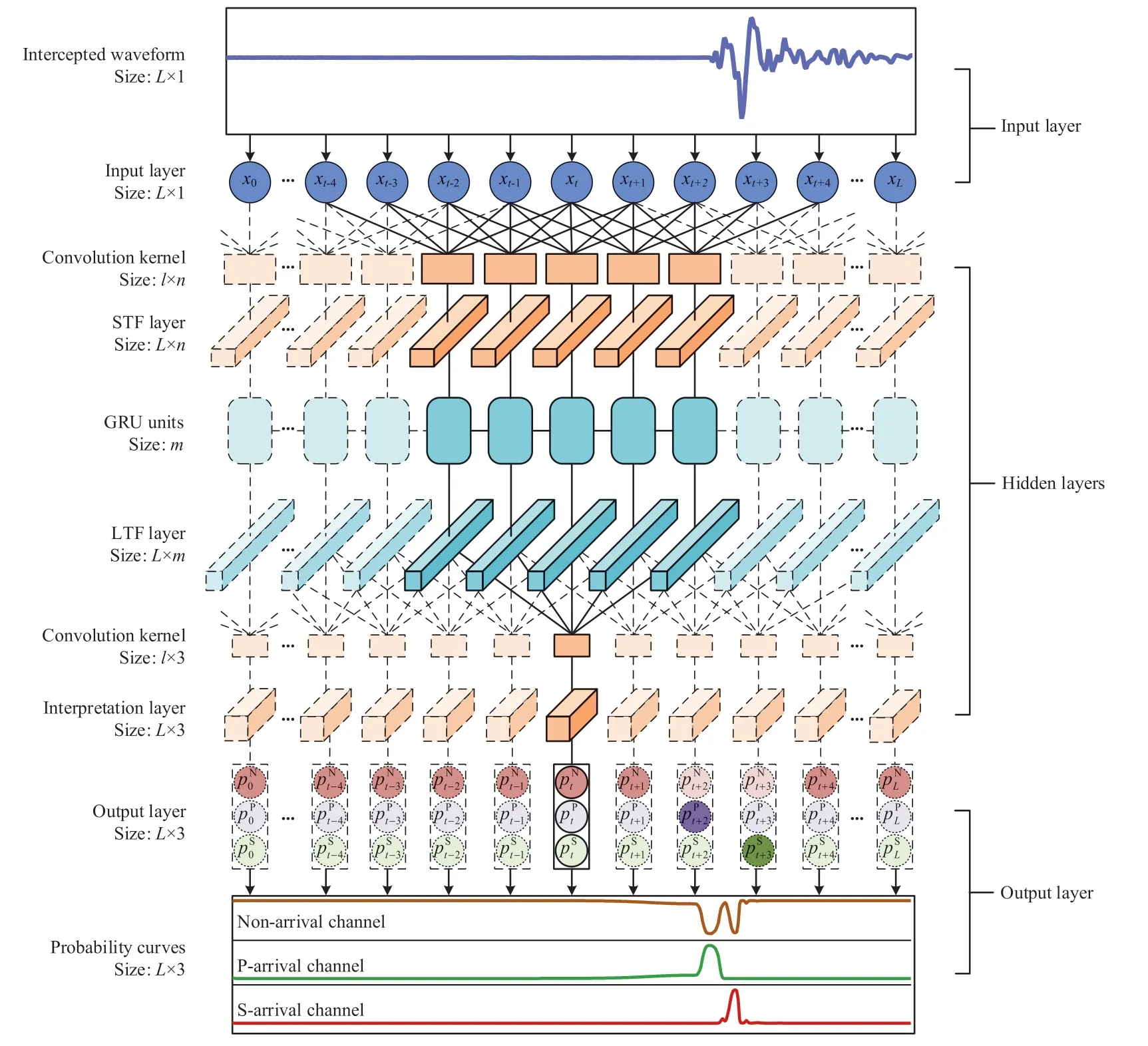
Fig.2.Structure of the CRNN model.L is the input waveform length,l is the convolution kernel width,n is the convolution channels,m is the GRU units,and the solid line area is the calculation process of the t-th sampling point (taking l=5 as an example in this context).
2.1.1.Input layer
The input of the CRNN model is original MS waveforms of rock mass microfracture signals,considering that deep learning models have a robust feature extraction ability.The need for additional filtering or transformation is non-essential,which would affect the real-time performance.However,it is necessary to normalize the input waveforms,considering that variations in rock fracture size and signal propagation distance can lead to considerable differences in the amplitudes of MS signals,which can even be as high as a factor of 103.The maximum absolute scaling method is used to linearly scale the MS signals to the range of[-1,1]to eliminate the influence of amplitude differences (Galli,2022):
where X′is the normalized input waveform,X is the original input waveform,max(•)is a function that outputs the maximum value of the argument,and abs(•) is a function that outputs the absolute value of the argument.
2.1.2.Hidden layers
The hidden layers are the key to the CRNN model.Three novel layers,namely the STF layer,the LTF layer and the interpretation layer,are designed to perfectly extract the features of P-and S-arrivals from rock mass microfracture signals,as shown in Fig.2.The STF layer uses a convolutional layer to extract the STF of MS signals,where the pooling layer is abandoned to maintain the length consistency of the inputs and outputs.The convolution kernel width (l) and convolution channels (n) are both important hyperparameters that affect the extraction of STF,and their values are determined through orthogonal tests.The calculation process of the convolutional layer is written as (Goodfellow et al.,2016).
The LTF layer uses a gated recurrent unit(GRU)(Bahdanau et al.,2014),which is a representative structure of RNN,to extract the LTF of MS signals.The GRU uses a reset gate and an update gate to realize information forgetting and updating,and uses state vector(ht) to store past information of MS signals before each sampling point,thus realizing the extraction of LTF with a small amount of computation,as shown in Eq.(3)(Goodfellow et al.,2016).The size of htis determined by the GRU units(m),which is also determined through orthogonal tests.
2.1.3.Output layer
Since the outputs of the interpretation layer range from 0 to positive infinity,there is a lack of contrast between the pre-and post-sampling points.The softmax function normalizes the interpretation layer outputs to a probability matrix pt=(Peterson and Söderberg,1989):
whereis the predicted probability of thek-th class at thet-th sampling point of the waveform,andktakes N,P and S,corresponding to non-,P-and S-arrival,respectively.
2.2.Optimization of the CRNN model
The arrival-picking task is essentially transformed into the classification of each sampling point using the CRNN model.However,because of the typically high sampling frequency(several kHz),MS waveforms are generally long time series,leading to extreme class imbalance and the loss of effective information.Thus,two corresponding optimizations of the CRNN model are proposed to accurately pick P-and S-arrivals of rock mass microfracture signals in real-time.
2.2.1.Waveform interception
Cho et al.(2014) showed that too long input sequences would reduce the learning performance of a GRU model and significantly increase the computational complexity,while too short input sequences will easily omit P-or S-arrivals and would be disturbed by changes in noise.When all other parameters remain unchanged,the effect of the input waveform length is studied to determine the appropriate value.The performance of the CRNN model is evaluated by the sum of the mean absolute errors for P-and S-arrivals(MAESUM):
whereTi,PandTi,Sare the automatically picked P-and S-arrivals of thei-th waveform,respectively;andare the real P-and Sarrivals of thei-th waveform,respectively;andNis the total number of waveforms.
As shown in Fig.3,with the increase of input waveform lengthL,the training time per epoch,the number of training epochs and the total training time show continuous increasing trends.More specifically,when the input waveform lengthLis in each of the three intervals (0,256),[256,1536] and (1536,4096],MAESUMshows a high value,a stable low value and a rapidly increasing value,respectively.This implies that the optimal value of the input waveform length is between 256 and 1536 sampling points.
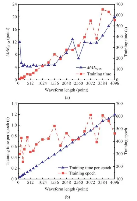
Fig.3.Influences of the input waveform length on the model training and picking accuracy: (a) MAESUM and total training time;and (b) Training time per epoch and training epochs.
In addition,two properties of the input waveform should be guaranteed: it should contain the arrival points of the P-and Swaves,and it should contain background noise of sufficient length.Thus,the waveform interception method is adopted:
whereTbandTeare the beginning and ending sampling points of the intercepted waveform,respectively;Tmaxis the sampling point corresponding to the maximum absolute amplitude,andTmax=argmax[abs(Xms)];Xmsis the time series of the MS waveform,Xms=[x1x2…xi],withxibeing the amplitude value of thei-th sampling point;aandbare the front and post amplification factors,respectively;and ΔTmaxis the maximum time interval between the P-and S-waves within the monitoring range,which can be obtained by (Zhu et al.,2022).
wherefsysis the sampling frequency of the MS monitoring system,lmaxis the maximum monitoring distance,and vP,vSare the wave velocities of the P-and S-waves,respectively.
Considering the Yebatan hydropower station project (YBT Project)as an example(see Section 4.1),the sampling frequency is 4000 Hz,the distance from each sensor to the edge of the monitoring area is between 200 m and 400 m,and the rock class in the project is mainly of grade III.Thus,it is assumed thatfsys=4000 Hz,lmax=300 m,vP=5500 m/s and vS=3500 m/s (Zhu et al.,2019;Li et al.,2021).We seta=3,where the length of 2ΔTmaxis used to learn the background noise information,and the remaining length is used to intercept the arrival information of the P-and S-waves.We setb=1 to prevent missing P-and S-arrivals.According to Eqs.(6)-(8),the input waveform lengthLis calculated to be 499,and is adjusted to 29=512 sampling points for convenience in deep learning processing.
2.2.2.Loss function
The loss function directly affects the gradient direction during model training (Dickson et al.,2022).The relative proportions of non-arrival,P-arrival and S-arrival sampling points are seriously imbalanced for MS arrival picking.To prevent the class imbalance from affecting the learning of minority classes (P-and S-arrivals),we introduced a class weightwfor P-and S-arrivals,and decomposed the loss into two parts:the average loss value at all sampling points(Lossall)(Zhu and Beroza,2019)and the average loss value at arrival points (Lossarr):
Through a comprehensive evaluation ofLossallandLossarr,it can be readily judged whether the model training direction is correct.The former evaluates the learning effect for the whole waveform without considering the class weight,whereas the latter evaluates the error between the predicted and actual values only at the actual arrival points of the P-and S-waves.Taking the waveform shown in Fig.4a as an example,Fig.4b shows that the model is too insensitive to respond effectively to the arrivals due to class imbalance,as indicated by the smallLossalland largeLossarr.In contrast,Fig.4c shows the case of a largeLossalland a smallLossarr,implying that the model is too sensitive and will incorrectly judge small waveform changes as arrivals.Fig.4d shows a divergent model with both a largeLossalland a largeLossarr.Only whenLossallandLossarrare small,as shown in Fig.4e,the model can achieve good performance.At this time,the model achieves a balance between robustness and sensitivity,picking the P-and S-arrivals correctly without the influence of noise.

Fig.4.Arrival picking results of the CRNN models with different Lossall and Lossarr:(a)The original waveform;(b) A small Lossall and a large Lossarr;(c) A large Lossall and a small Lossarr;(d) A large Lossall and a large Lossarr;and (e) A small Lossall and a small Lossarr.
Thus,during model training,Lossis used to guide gradient descent,andLossallandLossarrare taken as early stop criteria to avoid over-fitting issue: (1) the minimum value ofLossallis not updated for 20 consecutive epochs,and (2)Lossarr<0.1.
2.3.A real-time arrival picking method based on CRNN
The proposed real-time arrival picking method for rock mass microfracture signals consists of three modules: CRNN model training,real-time arrival picking,and dynamic feedback,as shown in Fig.5.

Fig.5.The flow chart of real-time arrival picking method based on CRNN.
2.3.1.CRNN model training
The steps for CRNN model training are as follows:
(1) Step 1: Select the training waveforms and mark the arrival points manually.The selected training waveforms should encompass rock mass microfracture signals with various amplitudes,frequencies and SNRs to enable comprehensive learning of the arrival features of various signals.
(2) Step 2: Label each sampling point of the waveforms with one-hot encoding.Non-arrival,P-arrival and S-arrival sampling points are marked as [1,0,0],[0,1,0] and [0,0,1],respectively.Each waveform corresponds to a sparse label matrix in chronological order,with a size ofL× 3.
(3) Step 3: Randomly initialize the weights of the CRNN model.
(4) Step 4:Input a training waveform into the CRNN model and output the corresponding probability matrix p=[ p1p2… pt… pL].
(5) Step 5: CalculateLoss,LossallandLossarraccording to Eqs.(9)-(11).
(6) Step 6: Use the Adam optimizer to update the CRNN model weights based onLoss.
(7) Step 7:Judge whether training is completed based onLossallandLossarr.End training if the conditions are met;otherwise,return to Step 4.
2.3.2.Real-time arrival picking
The steps for real-time arrival picking are as follows:
(1) Step 1:Monitor rock mass microfracture signals in real-time.
(2) Step 2:Calculate the recursive STA/LTA valueRof the current sampling point.
(3) Step 3:IfR>R0,whereR0is the trigger threshold,proceed to Step 4;otherwise,return to Step 1.
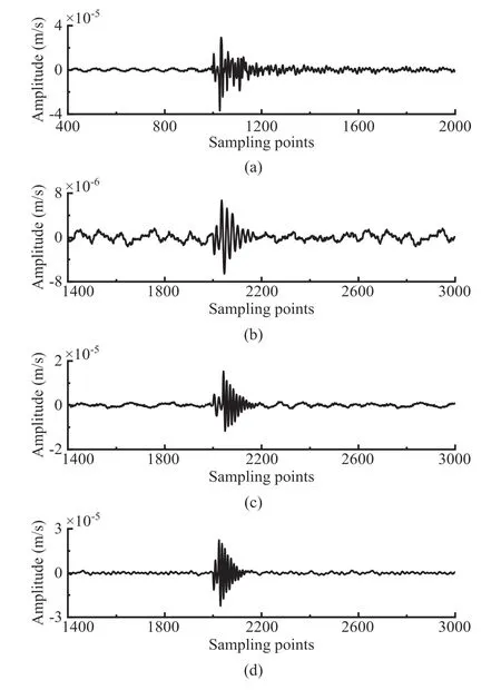
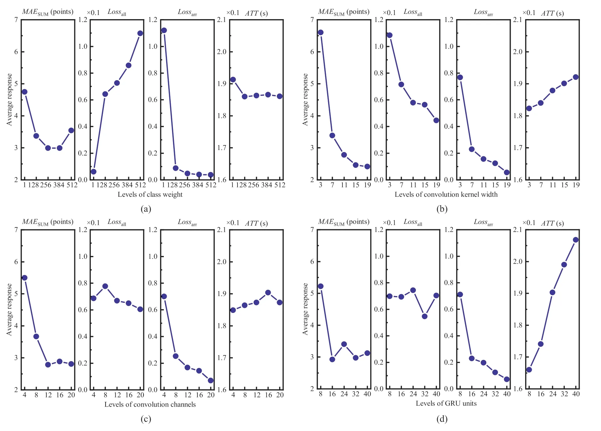
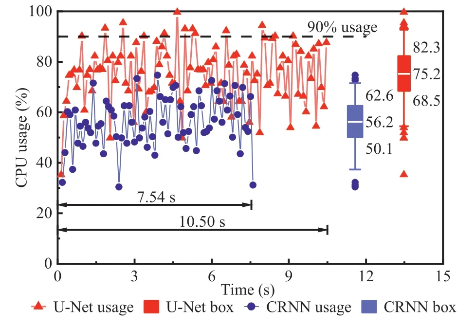
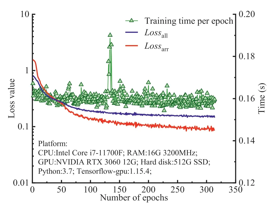
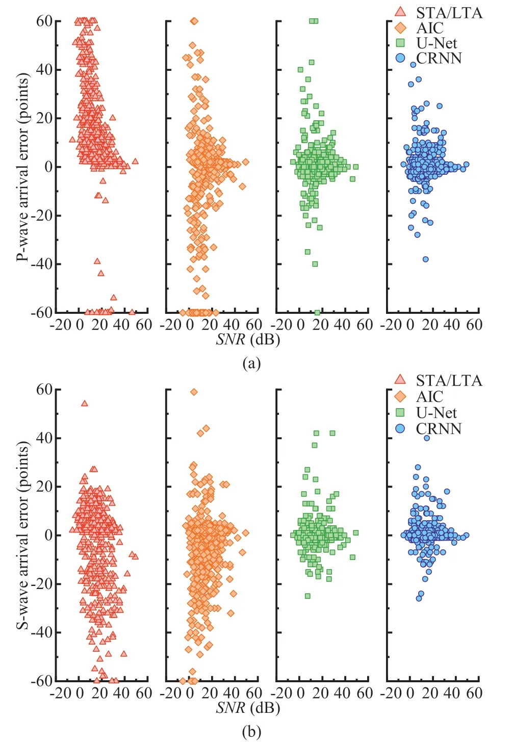
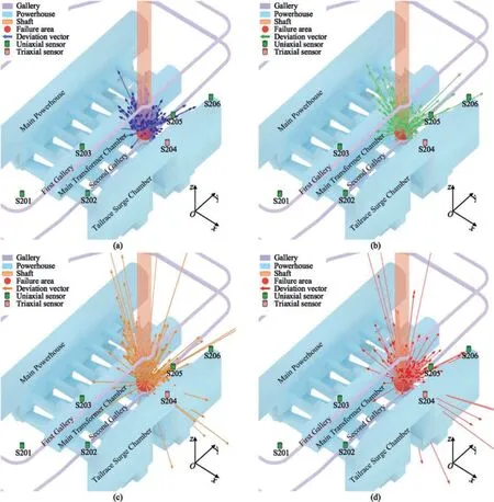
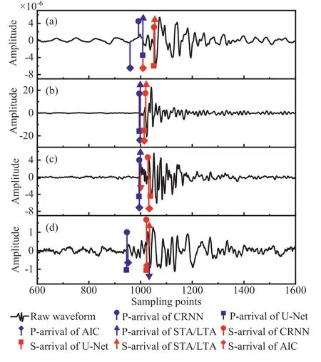
(4) Step 4:Record the MS waveform untilR (5) Step 5: Input the triggered waveform into the trained CRNN model and obtain the probability matrix. (6) Step 6: Take the sampling points corresponding to the maximum probability values of pPand pSas the P-and Sarrivals of the rock mass microfracture signal. 2.3.3.Dynamic feedback The steps for dynamic feedback are as follows: (1) Step 1:Regularly spot-check and calculate theMAESUMof the CRNN model.In particular,when the field environment,geological conditions or SNR changes significantly,it is necessary to evaluate the arrival picking accuracy of the CRNN model and calculate itsMAESUM. (2) Step 2:IfMAESUM≤MAE0,whereMAE0is an error threshold meeting the engineering requirements,the CRNN model is qualified and can be used to pick up arrivals of waveforms;otherwise,retrain the CRNN model with new MS waveforms under the current working conditions. Hyperparameters play an important role in the performance of deep learning models (Goodfellow et al.,2016).To optimize the performance of the CRNN model,four main hyperparameters were studied by combining simulation and orthogonal experiments:class weight,convolution kernel width,convolution channels and GRU units. 3.1.1.Experimental scheme Each hyperparameter is set with five levels,and the values corresponding to these levels are taken at equal intervals according to experience,as shown in Table 1.Thus,25 cases are designed in accordance with the orthogonal table L25(54)(Hedayat et al.,1999),as shown in Table 2.Four evaluation indexes are designed:MAESUM,Lossall,LossarrandATT.MAESUMis used to evaluate the picking ability of the CRNN model,calculated by Eq.(3),LossallandLossarrare used to evaluate the stability and sensitivity of the CRNN model,calculated by Eqs.(8)and(9),andATTis the time required for each training epoch,which is mainly used to evaluate the calculation speed of the CRNN model.Other hyperparameters of the CRNN model are also listed in Table 1. Table 1 Levels and values of hyperparameters in the CRNN model. Table 2 Orthogonal test scheme and corresponding responses. 3.1.2.Data preparation In view of the actual arrivals and controllable SNRs,the synthetic MS signals are the best choice to accurately evaluate the performance of the CRNN model.Different from other synthesis methods,we take real noises from the YBT Project as the background noise,and fully consider the characteristic distributions of the field MS signals such as the frequency,duration,and P-and Swave amplitude ratio.Then we use a Gaussian function to modulate the sine-basis function,calculated by Eq.(12).To ensure that the input noise does not contain potential valid signals,the real noise is defined as a continuous signal segment with STA/LTA values consistently less than 2.To prevent information leakage,the real noises do not include any data used in the engineering applications below.Typical synthetic MS signals are shown in Fig.6,which are highly similar to actual field signals.A total of 2500 MS signals were synthesized,including 1000 signals for training and 1500 signals for testing. Fig.6.Typical actual and synthetic MS signals of rock mass microfracture:(a)Real rock mass microfracture signal;(b) Synthetic signal with SNR=10 dB;(c) Synthetic signal with SNR=15 dB;and (d) Synthetic signal with SNR=20 dB. wheregN(t)is the real noise,AP,ASandANare the amplitude coefficients of the P-wave,S-wave and noise,respectively,andgP(t)andgS(t)are the sine functions of the P-and S-waves,respectively,modulated by a Gaussian function and calculated by whereTi,fiandli(i=P,S) are the arrival time,frequency and duration of the P-and S-waves,respectively. 3.1.3.Experiment results analysis To reduce the impact of the random initial weights on the training results,each case conducts 3 independent trainings with 3000 epochs.During training,we recorded theMAESUMof the test waveforms every 50 epochs,and finally selected the model corresponding to the minimumMAESUMamong the three independent trainings as the best model for each case.The test results of the 25 cases are shown in Table 2. Fig.7 shows a line graph of the responses to each hyperparameter based on intuitive analysis.The results show that: Fig.7.Average responses of evaluation indexes for each factor: (a) Class weight;(b) Convolution kernel width;(c) Convolution channels;and (d) GRU units. (1) In Fig.7a,with the increase of class weight,MAESUMfirst rapidly decreases to a minimum value and then increases;Lossallincreases continuously;Lossarrfirst rapidly decreases to a low level and then remains stable;andATTis basically stable throughout the process.Based on the discussion in Section 2.2,it can be found that the class weight is helpful to reduce the impact of class imbalance,but too large class weight will make the model too sensitive to STF while ignoring LTF,leading to incorrect arrival picking.In addition,the training time is not sensitive to the class weight.The suggested value of the class weight is 256. (2) In Fig.7b,as the convolution kernel width increases,MAESUM,LossallandLossarrfirst decrease and then tend to stabilize,whileATTincreases significantly.Considering the arrival picking accuracy and computational cost,the convolution kernel width is taken to be 15 in this context. (3) In Fig.7c,as the convolution channels increase,the trends of responses ofMAESUM,LossallandLossarrare similar to those of the convolution kernel width,whereasATTincreases slowly.The number of convolution channels is taken to be 12 in this paper. (4) In Fig.7d,with the increase of GRU units,MAESUMfirst quickly drops to a minimum and then begins to fluctuate;Lossallfluctuates within a consistent level;Lossarrcontinuously declines;andATTincreases rapidly.Once the value of GRU units exceeds a certain threshold,the arrival picking ability of the model is not significantly improved,but the computational cost greatly increases.Therefore,the number of GRUs units is set to 16 in this study. In general,the arrival picking ability of the CRNN model is significantly impacted by the convolution kernel width,followed by the convolution channels,GRU units,and class weight.GRU units have the greatest impact on the computational cost,followed by the convolution kernel width,which is consistent with the theory of CNN and RNN.An increase of hyperparameters can effectively improve the arrival picking accuracy at the cost of a greater computation.However,blindly increasing the hyperparameters will improve the CRNN model only to a limited extent,and may even cause over-fitting issue. 3.1.4.Performance verification Considering that the optimal hyperparameter configuration is not in the case of orthogonal test,we trained the CRNN model with the optimal hyperparameters to verify the optimization effect.The class weight,convolution kernel width,convolution channels and GRU units are 256,15,12 and 16,respectively.The training and test waveforms are the same as those in the orthogonal experiment,and the results are shown in Table 3.TheMAESUMof the optimized CRNN model is 2.26 points,which is smaller than that of any case in Table 2,and the arrival picking accuracy within 4 sampling points is excellent,which is 91.80% for P-wave and 98.73% for S-wave,respectively.Therefore,the orthogonal test correctly reveals the influence of each hyperparameter on the model performance,and the optimized model is defined as the standard CRNN model used below. Table 3 Results of arrival picking based on the optimized CRNN model. Computational performance is an important index to measure the ability of the CRNN model to pick MS signals in real-time.We compared the computational performance of the standard CRNN model and the typical U-Net model.In the U-Net model (Zhang et al.,2021b,2021c),the number of convolutional layers,convolution kernel width,convolution channels and the up-sampling rate are 5,7,[8,16,32,64,128] and 2,respectively.We used the trained CRNN model and U-Net model to pick arrivals of 100 batches(each batch has 100 waveforms),recorded the CPU usage of the models every 0.1 s,and calculated the average time per batch. Three multi-core computers with reduced performance and one single-core computer were selected to analyze the universality of the models.The computing performances of the CRNN model and U-Net model on each device are shown in Table 4.On the multicore CPU devices,both the CPU usage and average time per batch of the CRNN model are lower than those of the U-Net model,which are reduced by 30% and 25% approximately on average,respectively.With the decline in device performance,the gap in the CPU usage between the CRNN method and U-Net method decreases gradually,from 34.4%to 25.3%,and the gap in the average time per batch correspondingly increases,from 21.1% to 28.6%.In theextreme case of the single-core in device 4,both models fully occupy the thread,and the difference in the average time per batch is as high as 43.5%. Table 4 Computational performances of the two methods on different computers. Taking device 3 with low performance as an example,the CPU usage curve during arrival picking is shown in Fig.8.The U-Net model takes 10.50 s to pick arrivals,and the CPU usage is recorded 104 times,with values mainly between 68.46%and 82.30%.Taking 90%usage as the alert threshold,the U-Net model triggers the alert threshold 13 times,accounting for 12.5%of the total.It means that the U-Net method has almost reached the performance limit of device 3,which may affect the real-time acquisition and processing of MS signals,hindering the stable operation of the MS monitoring system.In contrast,the CRNN method takes 7.54 s to pick arrivals,where the CPU usage is mainly between 50.09%and 62.61%,and the maximum usage is only 74.69%.It shows that the CRNN method can work perfectly even on devices with limited performance,without affecting the normal operation of the MS monitoring system.Thus,compared with the U-Net model,the CRNN model has lower CPU usage,less computational cost and broader applicability. Fig.8.CPU usage curve during arrival picking on device 3. The YBT Project is located on the main upstream of the Jinsha River,at the junction of Baiyu County,Sichuan Province and Gongjue County,Tibet Autonomous Region,China.The underground caverns of this project are located in the Jinshajiang fault zone,with complex geological structures and developed faults.The surrounding rock is mainly of grade III quartz diorite.The uniaxial compressive strength is 120-180 MPa,and the measured maximum principal stress is 37.6 MPa.Relevant analysis shows the risks of rockburst,wall spalling,collapse and fault sliding during construction.Therefore,the SinoSeism (SSS) MS monitoring system,developed by Institute of Rock and Soil Mechanics,Chinese Academy of Sciences,and Hubei Seaquake Technology Co.,Ltd.,was deployed to monitor MS activity during the whole construction process.The monitoring system consists of 1 time server,1 data server,4 acquisition units,23 mono-component sensors and 3 three-component sensors.The sampling frequency is 4 kHz,the signal trigger algorithm is the improved STA/LTA algorithm,and the trigger threshold value is set to 4,instead of the more generally applied value of 6,to obtain more MS information of rock mass microfracture. A total of 1607 rock mass microfracture waveforms were collected from November 27,2021 to December 5,2021,803 of which were randomly selected for training,and the remaining 804 waveforms used for testing.The SNR and amplitude distributions ofall signals are shown in Fig.9.The SNR can be roughly estimated by Eq.(14).Fig.9a shows that the proportion of signals withSNR<10 dB among all signals is 25%.Fig.9b shows that the amplitude of 66%of the rock mass microfracture signals is lower than 10-5m/s,and this proportion increases to 93%for signals withSNR<10 dB.Thus,the waveforms from the YBT Project are typical weak rock mass microfracture signals,which are not conducive to picking Pand S-arrivals via traditional methods,such as the STA/LTA and AIC methods(Leonard and Kennett,1999;Dong et al.,2018). Fig.9.Characteristic statistics of rock mass microfracture signals from the YBT Project:(a) Distribution histogram of SNR,and (b) Scatter distribution of amplitude-SNR. wheres(t)andn(t)are the waveform data with 800 sampling points after and before P-arrival,respectively. To train a CRNN model suitable for picking up P-and S-arrivals of weak rock mass microfracture signals from the YBT Project,we first built the CRNN model structure as described in Section 2.1.Then,the synthetic waveforms were generated to obtain the optimal hyperparameters as described in Section 3.1.Finally the training field waveforms were input (see Section 4.1) to train the model weights via the Adam optimizer.The curves of the losses and time consumed during model training are shown in Fig.10.AlthoughLossarrstarts at a high level of 1.56 at the beginning of training,it decreases rapidly with the training and drops belowLossallafter only 45 epochs.At the same time,Lossalldeclined steadily and finally stabilized at approximately 0.14,without a trend of first decreasing and then increasing.The trends ofLossallandLossarrindicate that the class weight value is reasonable for highlighting arrival points,while also maintaining robustness for non-arrival points. Fig.10.Training losses and training time. The CRNN model completes its training at 314 epochs,with aLossallvalue of 0.14 and aLossarrvalue of 0.09.With NVIDIA’s CUDNN parallel computing platform,the average training time per epoch is only 0.16 s,and the total training time is 50.28 s.The results show that the CRNN model has an outstanding convergence speed and low training cost,meeting the demands of on-site monitoring. Considering that the actual arrivals of field MS signals are theoretically unobservable,the manually picked arrivals are approximately considered as the actual arrivals(Tan and He,2016).We defineA1as the picking accuracy of P-and S-arrivals within 4 sampling points,compared with the manually picked arrivals,andA2as the picking accuracy within 16 sampling points.The improved STA/LTA,AIC,trained CRNN and trained U-Net methods were used to pick the P-and S-arrivals of 804 test waveforms.The short-and long-term windows of the STA/LTA are 20 and 200 sampling points,respectively.The threshold is 5 for P-arrival and half of the maximum value for S-arrival,and the characteristic functions for Pand S-arrival(PCF(t)andSCF(t),respectively)are given in Eqs.(15)and(16)(Zhang et al.,2021b).The time window of the AIC is set to[Tb,Tmax] for P-arrival,and [TP,TP+αΔT] for S-arrival,where ΔTis the number of sampling points fromTPtoTmax,and α is a scale factor with a value of 1.2(Zhu et al.,2022).The hyperparameters of the U-Net model are shown in Section 3.2. TheA1accuracy,A2accuracy andMAEvalues for P-and S-waves are shown in Table 5.In terms of theA1accuracy,the CRNN method performs best,with 87.44% for P-wave and 91.29% for S-wave,followed by the U-Net method.The AIC and STA/LTA methods have a poor accuracy,especially the STA/LTA method,with 30.47% for Pwave and 39.18%for S-wave.For theA2accuracy,the CRNN and UNet methods have a similar performance,both exceeding 96%for Pand S-waves.The average accuracy of the AIC and STA/LTA methods increases to 82.34%,which is still generally lower than that of deep learning methods.In terms ofMAE,allMAEvalues of the CRNN are the lowest,with 2.57 sampling points for P-wave,1.66 sampling points for S-wave and 4.22 sampling points in total,followed by the U-Net method.The AIC method is slightly better than the STA/LTA method and inferior to the CRNN and U-Net methods.Additionally,the S-arrival picking accuracies of the four methods are generally higher than that of the P-arrival.This is because the low SNR of MS signals in the YBT project results in more noise interference on Pwaves than S-waves,which is consistent with the relevant study(Zhou et al.,2016;Fu et al.,2020). Table 5 Arrivals picking accuracy of each method. To compare the differences in the arrival picking results based on the four methods,the distributions of the arrival picking error and the change in the arrival picking error with SNR are calculated and shown in Figs.11 and 12,respectively.In Fig.11,the P-and Sarrivals picking errors of the CRNN and U-Net methods are characterized by‘symmetrical concentration’,that is,the picked arrivals are distributed evenly and symmetrically on both sides of the manually picked arrivals,mainly concentrated on the range of-4 to 4 sampling points.The AIC method has the characteristic of‘slight delay for the majority and extreme advance for the minority’for Pwaves,mainly concentrated within 8 sampling points.However,as the noise increases,arrivals can be easily triggered many sampling points in advance by the incorrect minimum points on the AIC curve,resulting in poor picking stability.For S-waves,the AIC method shows the characteristic of ‘scattered advance’,being mainly distributed between -16 and 4 sampling points.The STA/LTA method shows the characteristics of‘general delay’for P-waves and‘delay for the majority and scattered advance for the minority’for S-waves,mainly caused by its mechanisms of the sliding window and threshold-based trigger. Fig.11.Distributions of arrival picking errors based on the four methods: (a)P-arrival picking error,and (b) S-arrival picking error.The negative and positive errors mean that the picked arrival point is earlier and later than the manually picked point,respectively.Errors exceeding+32 and-32 sampling points are classified into[32,36]and [-36,-32] intervals,respectively. Fig.12 shows that as the SNR decreases,the P-and S-arrivals picking errors of all four methods tend to increase,but the CRNN and U-Net methods are less affected.In contrast,the AIC method performs well forSNR≥20 dB but sharply weakly forSNR<20 dB.The STA/LTA method shows high sensitivity to the SNR for P-arrival picking,and passivation for S-arrival picking. Fig.12.Scatter distributions of arrival picking errors with SNR based on the four methods: (a) P-arrival picking error,and (b) S-arrival picking error.Errors exceeding±60 sampling points are counted as ±60,respectively. Fig.13 presents the picking details for rock mass microfracture signals with 6 different SNRs.There is a general delay in P-and Sarrivals picking due to the average window of the STA/LTA method,and the degree of delay increases as the SNR decreases.WhenSNR<10 dB,as shown in Fig.13d,the P-arrival picked by the STA/LTA method lags behind the S-arrival,which indicates that the method can no longer distinguish the P-wave signal from the strong background noise.The AIC method has good picking accuracy,but its picking reliability depends on the quality of the input signals.Fig.13f shows the picking results when the input signal has a low SNR value and high background noise.The AIC method picks the Parrival in advance under the influence of the noise,and then incorrectly judges the real P-arrival as the S-arrival.The U-Net and CRNN methods can widely adapt to arrival picking under different SNR conditions.Nevertheless,it is worth mentioning that deep learning methods have a data-driven nature,which may lead to unexpected impacts of slight differences in the input signals.As shown in Fig.13d,the slight change in the background noise around the 950th sampling point is obviously reflected in the outputs of both the U-Net and CRNN methods.The difference is that the U-Net method misjudges it,while the CRNN method distinguishes the disturbance promptly and picks the real P-arrival.This is because the recurrent structure of the CRNN can naturally store all historical waveform information from the beginning,which can be used to combat noise.In contrast,the U-Net method only obtains the waveform information in a certain period before and after,through down-and up-sampling,lacking the ability to identify abrupt local changes. Fig.13.The arrival picking results of rock mass microfracture signals with different SNRs:(a)SNR=25.4 dB;(b)SNR=19.1 dB;(c)SNR=15.1 dB;(d)SNR=8.0 dB;(e)SNR=5.1 dB;and(f)SNR=2.2 dB.ΔP and ΔS are the difference between the picked P-and S-arrivals,respectively,and the manually picked arrivals.Negative numbers represent an advance,and positive numbers represent a delay. In summary,it can be found that the CRNN method has the highest accuracy,the lowestMAEvalues,and a strong antiinterference ability for both P-and S-waves.The U-Net method is inferior to the CRNN method slightly in various indicators,which is relatively similar but superior to the STA/LTA and AIC methods.For the two traditional methods,the AIC method has higher accuracy but poorer stability,and is sensitive to noise.The STA/LTA method has lower picking accuracy but better stability,which is consistent with the existing research results (Shang et al.,2018). In view of the analysis in Section 4.3,during the MS monitoring for rock-mass stability of the YBT Project construction,the CRNN method has been used to pick P-and S-arrivals in real-time.Then the Newton second order,Newton downhill method (Li and Chen,2013),was used to locate the rock mass microfracture in order to evaluate the stability of the rock mass. During the monitoring process,rock mass microfracture signals occurred in the junction area between the shaft and the second gallery on March 19,2022.As of March 31,183 rock mass microfracture events had been accumulated in this area.A cloud diagram of the spatial distribution density is shown in Fig.14.Fig.15 shows the evolution of the microfracture events with time,implying that rock mass microfractures with moment magnitudes (Mw) mainly ranged from -1 to -0.5,and continued to occur in this area,especially on March 28.According to on-site feedback,three faults(F85,F88 and F21)pass through this area,leading to poor integrity of the rock mass in the faults and the adjacent areas.The maximum in situ stress in the fault area is 12.5-18.8 MPa,and the maximum in situ stress between the faults with good rock mass integrity is 37.6 MPa.On March 30 and 31,2022,multiple failures occurred in the area between the faults,which were mainly stress-type spalling failures.The spalled rocks are mainly thin blocky or thin flaky rocks,with fresh and unfilled failure surfaces,as shown in Fig.16.It shows that,in terms of weak microfracture events withMw<-0.5,the positioning results based on the arrivals picked by the CRNN method have a good consistency with the actual failures,providing a good support for engineering construction. Fig.14.Density nephogram of microfracture events based on the CRNN method (March 19-31,2022). Fig.15.Evolution trend of microfracture events with time based on the CRNN method(March 19-31,2022). Fig.16.Rock mass failure at the junction area between the shaft and the second gallery. To analyze the positioning differences of the various methods,the CRNN,U-Net,AIC and STA/LTA methods are used to pick P-and S-arrivals,and 183 rock mass microfracture events in the shaft area are recorded.The measured coordinates of the surface failure are used to approximate the actual location of the failure occurring within the rock mass.The deviation vectors are defined as directed line segments that start from the center of the failure area and end at the MS positioning results,as shown in Fig.17.Fig.18 shows the sets of deviation vectors calculated by each method.In terms of the macroscopic distribution of MS sources,all four methods show a trend of roughly distributing along theXOZplane of the failure area.Meanwhile,most microseismic events are distributed above the second gallery,rather than being symmetrically distributed along the failure center.This is because that this area was undergoing pilot drilling upwards before failure occurred,and the incubation of microfracture inside the rock mass promoted the occurrence of apparent failure.Among these four methods,the deviation vectors of the CRNN method are the most concentrated and closest to the failure center,followed by the U-Net method.Although the deviation vectors of the AIC and STA/LTA methods are also concentrated in the failure area overall,they are more scattered than those of the two deep learning methods.The positioning results of the AIC method are the most divergent,which is significantly affected by SNR.As shown in Fig.19,the deep learning methods pick up the arrivals at the same precision regardless of the SNR.The STA/LTA and AIC methods have a good performance with high SNR,while have an unstable trend with low SNR.The difference is that the STA/LTA method tends to pick up P-waves with hysteresis so that the Pand S-arrivals overlap,as shown in Fig.19c and d.The overlapping results in positioning algorithms based on the arrival time differences positioning the source near the sensor array.However,the AIC method tends to pick up P-waves in advance,as shown in Fig.19a,leading to significant arrival time differences,seriously affecting positioning accuracy and even causing positioning divergence. Fig.17.Schematic of deviation vectors. Fig.18.Deviation vectors from the failure center to the positioning results:(a)CRNN method;(b)U-Net method;(c)AIC method;and(d)STA/LTA method.S201-S206 are the MS sensors arranged near the failure area. Fig.19.Arrival picking results for different waveforms of the same microfracture:(a)-(d) are the waveforms of the same microfracture monitored by different MS sensors. Table 6 presents the average distances of the 183 microfracture events from the calculated location to the failure center.The average distance of the CRNN method is 28.79 m,which is the smallest among the four methods,indicating that the CRNN method picks arrivals stably and reflects the on-site failures well.The U-Net method is slightly worse than the CRNN method.The average distances of the AIC and STA/LTA methods are greater than 50 m,larger than that of the deep learning methods.In addition,the average distances of all four methods show a trend that can be characterized as the order ofZ-axis >X-axis >Y-axis.This is because the MS sensors were mainly distributed in the first gallery due to the spatial structure and construction progress when failure occurred.The microfracture events were mostly outside the sensor array inZ-axis direction,leading to greater positioning error inZaxis direction (Feng et al.,2015;Chen et al.,2021). Table 6 The average distances from the calculated location results to the failure center. To address the common contradiction between accuracy and computation in the current arrival picking methods,a real-time arrival picking method based on CRNN is proposed.The hyperparameter sensitivities,computational performance and arrival picking accuracy of the proposed method are analyzed based on synthetic and field MS data,and the proposed method has been applied to the YBT Project for MS monitoring.The conclusions are drawn as follows: (1) The hyperparameters have a significant impact on the performance of the CRNN model.An increase of hyperparameters can effectively improve the arrival picking accuracy at the cost of more computations.However,blindly increasing the hyperparameters only shows a limited improvement and may even cause over-fitting issue.The hyperparameters with the most significant impacts on arrival picking ability and computational cost are the convolution kernel width and GRU units,respectively. (2) The computational performance of the CRNN method is better than that of the U-Net method,showing average decreases of 30% and 25% in CPU usage and average time per batch,respectively,implying a broader applicability of the CRNN method. (3) Compared with the STA/LTA,AIC and U-Net methods,the CRNN method has the highest picking accuracy,the lowestMAEvalues,and a strong anti-interference ability for both Pand S-waves.Within 4 sampling points,the accuracy of the CRNN mothed is 87.44%for P-arrival and 91.29%for S-arrival,both of which exceed 96%within 16 sampling points,and theMAESUMis only 4.22 points,followed by the U-Net,AIC and STA/LTA methods. (4) In the application of YBT Project,the positioning results based on the arrivals picked by the CRNN method show the best consistency with the actual failure zone,followed by those of the U-Net,STA/LTA and AIC methods,thus proving the reliability of the CRNN method in engineering applications. Declaration of competing interest The authors declare that they have no known competing financial interests or personal relationships that could have appeared to influence the work reported in this paper. The authors declare the following financial interests/personal relationships which may be considered as potential competing interests: Acknowledgments We acknowledge the funding support from National Natural Science Foundation of China (Grant No.42077263).3.Performance analysis
3.1.Impact of hyperparameters on model performance



3.2.Computational performance analysis

4.Application
4.1.Engineering background

4.2.Model training
4.3.Picking results analysis



4.4.Application in field failure monitoring



5.Conclusions
 Journal of Rock Mechanics and Geotechnical Engineering2024年3期
- Journal of Rock Mechanics and Geotechnical Engineering的其它文章
- Using deep neural networks coupled with principal component analysis for ore production forecasting at open-pit mines
- Sliding behaviors of the trapezoidal roof rock block under a lateral dynamic disturbance
- Failure characterization of fully grouted rock bolts under triaxial testing
- Nonlinear constitutive models of rock structural plane and their applications
- Mechanical behaviors of backfill-rock composites:Physical shear test and back-analysis
- Slope stability of reclaimed coal mines through a new water filling index
