Deployment of Edge Computing Nodes in IoT:Effective Implementation of Simulated Annealing Method Based on User Location

Junhui Zhao ,Ziyang Zhang ,Zhenghao Yi ,Xiaoting Ma ,Qingmiao Zhang

1 School of Electronic and Information Engineering,Beijing Jiaotong University,Beijing 100044,China

2 School of Information Engineering,East China Jiaotong University,Nanchang 330013,China

Abstract: Edge computing paradigm for 5G architecture has been considered as one of the most effective ways to realize low latency and highly reliable communication,which brings computing tasks and network resources to the edge of network.The deployment of edge computing nodes is a key factor affecting the service performance of edge computing systems.In this paper,we propose a method for deploying edge computing nodes based on user location.Through the combination of Simulation of Urban Mobility(SUMO)and Network Simulator-3(NS-3),a simulation platform is built to generate data of hotspot areas in IoT scenario.By effectively using the data generated by the communication between users in IoT scenario,the location area of the user terminal can be obtained.On this basis,the deployment problem is expressed as a mixed integer linear problem,which can be solved by Simulated Annealing (SA) method.The analysis of the results shows that,compared with the traditional method,the proposed method has faster convergence speed and better performance.

Keywords: deployment problem;edge computing;internet of things;machine learning

I.INTRODUCTION

With the large scale deployment of 5th Generation Mobile Communication Technology (5G) networks,the information society has been rapidly changing from the pure Internet to the Internet of Things(IoT),and human society has gradually entered the mode of interconnection of all things [1,2].The advanced communication and bandwidth capabilities of 5G can meet the requirements of high-reliability connections for IoT applications and contribute to the development of the IoT[3,4].IoT gives access devices the ability to see,listen,and think through communication technologies,Internet protocols,and applications,turning these physical devices into intelligent objects.With the help of cloud computing big data and mobile Internet,the combination of digital and physical world is realized [5].According to the Cisco Report Visual Network Index (VNI),the number of global mobile devices will grow to 13.1 billion by 2023,of which 1.4 billion will support 5G,and the number of 5G devices and connections will account for more than 10 percent of global mobile devices and connections [6].More and more physical devices and virtual devices are connected to the network at an unprecedented speed,and information is exchanged in the network to achieve information sharing,which is also the ultimate concept of IoT[7].

With the ultra density access of IoT devices,the IoT has ushered in arduous challenges in terms of low latency and highly reliable connections [8,9].For example,the smart medical system based on IoT puts forward higher requirements for reducing system delay and ensuring network security,so that the effect of telemedicine is closer to traditional medical treatment.Moreover,the relay protection of the smart grid requires a minimum delay of 15 milliseconds;industrial control requires a delay of 1 to 10 milliseconds;and automatic driving technology requires a minimum delay of 3 to 5 milliseconds.Therefore,as the basic guarantee conditions for the construction of smart cities,communication networks are faced with upgrades and transformations in terms of reducing delays and improving the reliability of network connections.Due to the increasing number of devices and growing diverse demands of different services,achieving efficient use of resources remains challenging,and methods must be developed to meet the emerging needs of IoT [10].Improving hardware is a proper method to reduce delay [11],but we usually sink business functions located on the network cloud to the edge of the network,and as close as possible to the data source location.Besides,big data can be used to effectively standardize and optimize edge computing nodes,improve the system capacity and operating efficiency of IoT systems,and reduce data processing delays.

Mobile Edge Computing(MEC)can bring network service business to the edge of the network,establish a server between the service user and the service host,and complete network tasks[12].Edge computing nodes are usually deployed in remote data centers and close to clients.In IoT systems,it is unquestionable that the tasks need to be offloaded to the edge of network.In addition,critical communications that are sensitive to delay and interference from the surrounding environment add much complexity because they require top-notch reliability and availability while ensuring ultra-low latency.As is shown in Figure 1,MEC can be applied to various scenarios such as IoT,smart cities,and smart transportation.The service delay of communication channels can be minimized by setting the network service facilities to the edge of the network,and thus MEC becomes the core solution to these problems.

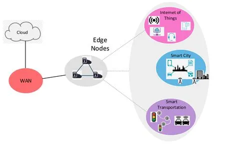
Figure 1. Mobile edge computing deployment diagram.

MEC technology attempts to build a computing resource environment close to the user,which is the Radio Access Network(RAN).RAN has the advantages of high performance,high bandwidth,high reliability,and low latency for some IoT applications.To ensure the complex data processing and low-latency communication requirements of the future cellular IoT,how to scientifically and reasonably deploy edge computing nodes is an urgent problem needed to be tackled.Therefore,it is necessary to use big data analysis to learn the interference,load,traffic,and the number of daily access devices in the edge computing nodes of the existing cellular IoT micro base stations in a certain area.Under the criterion of delay,the deployment requirements of edge computing nodes in a certain area can be modeled.The established edge computing deployment requirement model is more accord with the communication demands of the cellular IoT in the set area,in which the communication delay of the entire system can be greatly reduced.Besides,it is necessary to reduce communication costs and communication resource occupation in edge computing [13].Due to the distributed nature of edge computing,a certain number of edge computing nodes need to be deployed in a certain cellular IoT network area,the deployment costs and operating costs have become the key issues.By optimizing the selection of edge computing nodes,deployment and maintenance costs can be greatly reduced.However,due to the large number of trade-offs involved,such as the communication needs of hot spots in the cellular IoT,deployment solutions are usually difficult to obtain.Therefore,a method for deploying edge computing nodes based on user location is proposed in this paper.The main contributions of this paper are summarized as follows:

• Based on the prediction information and user node movement model,a general edge computing node deployment scheme is designed,which can dynamically adjust the layout strategy according to the changes of end user nodes.

• In the proposed edge computing nodes deployment scheme,the changes in communication scenarios and models of connection costs,operating costs,and delay costs are considered to make the results more realistic and reliable.

• Using the regional positioning prediction model,the main parameters of the optimal configuration strategy for edge computing nodes are realized,and the dynamic allocation of edge nodes to computing resources is realized.

• Based on the prediction parameters,a set of edge computing node deployment algorithms based on Simulated Annealing (SA) is proposed to ensure the optimal layout strategy of edge computing nodes,including the location of edge computing nodes and the resource allocation of each edge computing node.

This article is organized as follows: Section II introduces related work and problems faced.In Section III,the system model of this paper is proposed.Section IV mainly introduces the preparations for experimental simulation and summarizes the framework scheme with its main features,Section V presents the evaluation results of edge computing node deployment,and the conclusion is summarized in Section VI.

II.RELATED WORK AND FACED PROBLEMS

The deployment of IoT edge computing nodes is the basic condition for completing the research on key technologies for future communication networks with low-latency,high-reliability IoT technologies.User terminals in the IoT have strong mobility,randomness,periodicity,non-stationarity,and spatial correlation,which not only causes changes in network topology,but also puts forward stricter requirements for low latency and high reliability of network connections.At the same time,when considering the distributed characteristics of edge computing and the large number of edge computing nodes which to be deployed,cost of deployment and operations is also a key issue to be faced with.In this case,research on deployment schemes of edge computing nodes becomes crucial.In this part,we summarize the existing research work.

Cloud computing is one of the most effective methods for processing big data.However,cloud computing resources are usually concentrated in mainframe computers of data centers which is away from most cellular IoT terminals.Therefore,there could be high latency between the IoT terminal and the cloud,reducing the processing rate of the data,and consuming a lot of bandwidth resources.In order to solve these problems,Satyanarayanan et al.in[14]proposed edge computing so that the edge access network can compute and store resources.In[15–17],researchers had pointed out that edge computing can be used to shift workloads from a centralized cloud to the edge of network,improve response time and save network resources.

Some researchers have realized that the generated data can be hosted on the edge network to achieve low-latency data processing in the Internet of Vehicles.Mach et al.in[18]introduced the framework of MEC and proposed how to balance low-latency user requirements and reducing power consumption.In [19],the authors solved the problem of effective deployment of edge computing nodes in smart cities,and introduced a mixed integer linear programming formula that can minimize the deployment cost of edge devices by meeting the goals of network coverage and computing user traffic requirements.The proposed method can accurately model a complex urban environment with many buildings and a large number of vehicles.In [20],the authors proposed a flexible and mature edge computing architecture to support Internet of Vehicles services with strict latency requirements.At the same time,it focuses on the extended virtual sensing service,which aims to use the data collected by the network infrastructure to enhance the sensor measurement on the vehicle,and use this information to obtain better safety and improve the comfort of passengers or drivers.

However,these studies have not considered the diversity of user node traffic data types in edge computing.The business types and requirements of the existing user nodes mostly depend on the probability distribution of user nodes.There is no comprehensive analysis of the characteristics of user traffic data.Besides,the parameter assumptions are ideal in those papers,and it would be better to built system model for the real scenarios.Simultaneously,with the increase of the feature variable of user node data,the existing user node traffic model is difficult to reasonably classify and process these data,thus the high reliability and low delay communication can not be guaranteed.

In [21],the author proposed a solution for edge server deployment,with the goal of optimizing the service performance and operating cost of the edge infrastructure.The main difference from traditional server deployment methods is that the proposed method can find unpredictable edge deployment locations,thereby reducing the cost of edge configuration more comprehensively and efficiently.In[22],the author considered an MEC system with multiple users,which combines 5G and MEC.In the proposed solution,a base station with an MEC server can not only provide computing offloading services,but also provide data caching services.In[23],the authors solved the problem of effectively deploying a limited number of edge nodes in urban scenarios under a limited budget.They used a 5G architecture edge computing paradigm,in which storage,computing,and network resources are brought to the edge of the network.The effectiveness of vehicle applications is directly related to the correct deployment of edge nodes.The authors in[24]proposed an edge computing node deployment scheme with dynamic virtual functions,which can generate edge node deployment strategies based on prediction information.The proposed layout plan uses cloud computing pay-as-you-go and competitive instance models,which can easily and flexibly allocate service resources with low cost.In [25],the author optimized the system cost by considering the calculation price,energy consumption and delay together.By minimizing the system cost,an intelligent shunting strategy based on ant colony optimization algorithm was proposed,in which the ants randomly visit computational access points to obtain the final result.

The above research results all reflect the superiority of edge computing,but when it is specifically applied to IoT,the existing node deployment schemes lack the optimization analysis of the Internet of Things user data.According to the business needs of IoT users in different industries,it is necessary to obtain accurate user types and behavior portraits by analyzing user data,and then obtain the deployment requirements of edge computing nodes.Since the edge network is closer to the terminal of IoT,the real data of the terminal can be obtained in real time,and these data have full dimensions,including parameters such as location,time,and behavior.After analyzing these more reliable data,accurate information such as the time and distribution of various behaviors of IoT terminals can be obtained,and then implement customized service with low-latency and high reliability through customized edge computing node deployment.

In order to ensure that the future IoT can handle complex data and meet the requirements of low latency and high reliable communication,edge computing nodes need to be deployed scientifically and reasonably.In this paper,big data analysis is applied to learn the interference,load,traffic and daily average number of access devices in a certain area.Under the guidelines of maximizing throughput and minimizing communication delay,the deployment requirements of edge computing nodes in a certain area are modeled based on the real scenarios.The established edge computing deployment requirement model is more in line with the communication requirements of the cellular IoT in the set area,which greatly reduces the communication delay of the entire system.

III.SYSTEM MODEL

In this section,an innovative point of deploying edge computing nodes in the IoT is based on the data generated by user nodes in a network scenario.Data mining technology is used to mine the business needs of different industries and different IoT terminals in the network.This learning method obtains accurate user types and behavior trajectories,and obtains hot spot distribution of user nodes’communication areas in the IoT,which provides a foundation for the deployment of edge computing nodes.

In this part,we first build a cellular IoT network.Then,according to the Signal Interference plus Noise Ratio(SINR)value between the user node and the base station,a neural network is used to train the location area.The obtained training model can locate the user equipment in the location area,thereby determining the number of edge computing node devices in the IoT network.Finally,an optimization model for edge computing nodes is proposed,and the optimal deployment area is determined by SA algorithm[26].

3.1 Cellular IoT System Model

The accurate IoT terminal network model can not only improve the authenticity of the prediction model,but also help the smooth completion of the deployment of edge computing nodes.We set Beijing,China as the target area for the deployment of MEC services,because it has a complex network environment,diverse user business types and a large amount of communication data.From OpenStreetMap,we get a map of the center of Beijing,which contains information such as roads and buildings.It provides a good simulation environment for user nodes with multiple business functions.We select a part of XiDan commercial district covering an area of 1.5 times 0.8 square kilometers as our simulation area.After that,we use the tools provided by Simulation of Urban Mobility (SUMO)to extract road networks and buildings to generate a simulation environment.In SUMO simulation platform,the impact of buildings is not considered.The area surrounded by red lines in Figure 2 shows the map of the considered deployment area.In the simulation area,user terminals such as pedestrians and vehicles send communication data to the nearby base station,and then access the core network after processing by the MEC server.

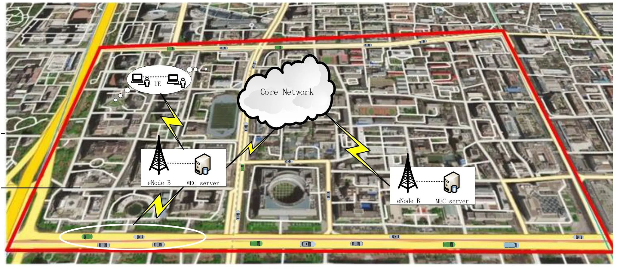
Figure 2. Traffic models of user terminals with different business functions.

Then in the Network Simulator 3 (NS-3),the user node behaviors generated by SUMO are combined to build a cellular IoT network model.This model takes into account the communication obstacles caused by the existence of the building,and considers the material,structure,height and other factors of the building,which is ideally suited for the dense structure of the deployment area.NS-3 can bind traffic trajectories generated from SUMO to user nodes,and can edit the messaging protocol standards of user nodes.In the network environment,the type and size of buildings can be added to affect the transmission of communication,so as to be closer to the real scene.In addition,NS-3 can simulate events such as signal transmission conflicts and low signal strength,which will cause information loss.

In the simulation,the communication between the vehicle and the eNB refers to the IEEE 802.11p standard.The eNB transmit power level is set to 23 dBm.The communication vehicle and user terminal send a message every second with a payload of 1040 bytes.The key parameters and related values used in the NS-3 simulation are shown in Table 1.

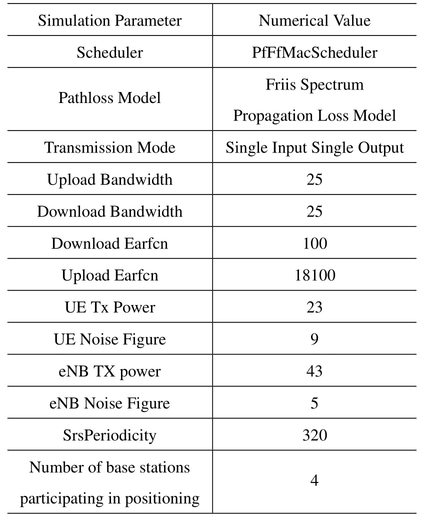
Table 1. NS-3 network parameters.

3.2 Positioning System Model

We use NS-3 platform for communication simulation.In the simulation process,we will consider the interference of the complex environment,such as the occlusion of buildings and the fading type of the selected channel,which will lead to a large uncertainty in the signal strength received by the user node.SINR can measure the quality of the connection link between the user node and the base station,so the value of the SINR can be selected as a parameter for locating the user node.After setting the network environment according to the parameters in Table 1,the SINR values collected by NS-3 are initially processed and used as the input of the neural network training model,and the actual location area of the user node is used as the output result of the neural network training model.After three layer neural network training,the positioning model is obtained.

We use feed-forward neural networks to train the localization model [27].The neural network collects a large number of known inputs and outputs and selects a learning process to train these data.Generally,a certain learning algorithm can be used to find the nonlinear relationship between input and output.Then,use this relationship to build a neural network learning model.Finally,use the trained model to predict the output based on the new input,and judge the effect of the model based on the output result.

According to the amount of data collected by user nodes and the complexity of the communication network environment,we have added three hidden layers to the Hiddenlayer of the neural network.The nodes of each layer are called neurons in the neural network.

We considered back propagation (BP) neural network,which is a neural network learning algorithm with supervised learning.In this neural network,each neuron is only connected to neurons in adjacent layers.The BP neural network will analyze the error between each training result and the expected result,and then modify the weight and threshold iteration to obtain a model that can gradually output consistent with the expected result.

The algorithm learning process is mainly divided into neural transmission and weight update.

In the process of neural transmission,the input signal is connected to the output node through the hidden layer,and the output signal is generated after the nonlinear transformation.When the actual output does not match the set output,the actual output will be compared with the expected output to generate an error,and then the error will be propagated back.Given the training set [(x1,y1),(x2,y2),...,(xn,yn)],where xi∈RI,yk∈RK.It means that the input example consists of I attributes,and the output is a K dimensional variable.The hidden layer is denoted by[h1,h2,...,hJ].Then the jth hidden layer neuron hjand the kth output layer neuron ykare computed by

The activation function introduces a nonlinear factor to the neuron,so that the neural network can approach any nonlinear function arbitrarily.In this paper,we used the Sigmod function,which can transform the input signal between negative infinity and positive infinity into an output between 0 and 1.The activation function is defined as

In the process of the update of the weights,the output errors are gradually transferred back to the input layer through the hidden layer,and these errors are distributed to all neurons in each layer.The weight adjustment is based on the size of the error value obtained in each layer.In a training example (xn,yn),the threshold of the kth neuron in the output layer is represented by θk.Suppose the training output of the neural network is,where

Then the error of this prediction result can be expressed by the least square method:

The next step is to adjust the values of the parameters of each layer according to this error,and reduce Enstep by step.In summary,we can know thatfirst affects βk,then,and finally En,so we can get:

where η is training speed,

Using the same method,update the weights of the input layer and hidden layer.The neural network training ends when the error reaches an acceptable range.

3.3 Edge Computing Node Optimization Model

In order to formulate an edge computing node deployment plan restricted by low latency and high reliability,user nodes with different service types distributed in a given area are modeled as traffic generators as shown in Figure 3.Edge computing node locations are set to a Mixed Integer Linear Problems (MILP),which is the main goal of optimizing the invest of the entire edge network network.Table 2 summarizes the notation used in the optimization model.

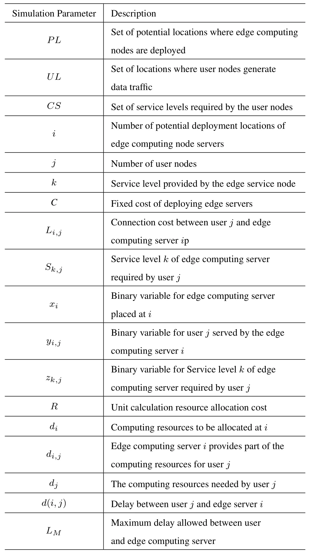
Table 2. Simulation parameters.

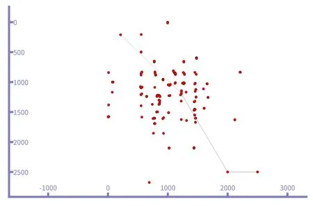
Figure 3. Map describes service user locations and hot spots.

This model requires some assumptions to simulate various display challenges.First of all,the transmission delay is assumed to be the transmission delay between the serving user and the base station,and the processing delay can be obtained from the trance file generated during the NS-3 simulation process.Secondly,because the nature of the problem is combinatorial,in order to reduce the calculation time and make the MILP formula solvable,we assumed that the initial edge nodes are randomly generated and the position coordinates are known.And then,in the simulation process,the data transmission rate and the amount of data to be transmitted are different for each user.We use the NS-3 LTE module to configure the parameters.Finally,according to the requirements of 5G,a delay of 10ms is selected as the maximum coverage of the edge node (i.e.,LM=10ms).For the tasks with lower latency,we take another restriction.Our optimization goal is to minimize the deployment cost of edge computing nodes under the condition that the terminals can communicate well with edge computing nodes in the IoT scenario.Therefore,the optimization problemP1is formulated as:

The optimization objective function in (10a) represents the cost to be considered for deploying edge computing servers.The first term is the fixed cost of deploying edge computing servers,which is mainly related to the number of edge computing servers.We determine the number of edge computing servers based on the number of users in the hotspot area.The second term represents the cost required for each user to connect to the edge computing server serving him,which is mainly related to the delay of data transmission and processing.The data can be obtained through the trace command of NS-3.The third term is the service level demand cost,which is mainly related to the business type of user nodes.For example,for vehicle user nodes and mobile device nodes in the IoT scenario,the corresponding k values are different,and the service Sj,kprovided by edge computing nodes are also different.The fourth term is the cost of edge computing node resource configuration,which is mainly determined by the type of user node and the amount of data transmission.In the communication data simulation stage,use the LTE module in NS-3 to configure different data transmission rates for mobile device nodes or vehicle user nodes,and use trace commands to obtain processed data.

The constraint in (10b) allows an edge computing server to be deployed at location i only if there is at least one user in UL within its coverage range,which is determined by the location of edge computing nodes in the previous work.As any user node in UL can be covered by one or more edge computing nodes in PL,the constraint condition (10c) reflects that the sum of the computing resource allocation provided by all the covered edge computing nodes must be equal to the total computing resources of the user node demand.After that,the edge computing node in PL which provides computing resources to user nodes in UL meets the constraint (10d),the computing resources allocated by edge computing node at i to user node at j cannot exceed the maximum capacity that i can provide.The constraint (10e) describes the relationship between the computing resources required by the user node at j and the edge computing node deployed at i,which is restricted by yi,j.Moreover,in the constraint(10f),if the user node at j is not covered by the edge computing node at i,the computing resource demand between i and j is forced to zero.Similarly,in constraint(10g),if edge computing node is not placed at i,then there is no computing resource demand for any user nodes at this location.When the user node at j is connected to the edge computing server at i,the delay between them is determined by constraint(10h).User node constraints are restricted by formula(10i).(10j)limits the value range of the parameters and expresses the decision variables as binary integer variables.

IV.EXPERIMENTAL SIMULATION AND FRAMEWORK OVERVIEW

This section first collects and preprocesses the data as an input part of the entire system model.Then the data evaluation method is introduced.Finally,we make a reasonable analysis of the simulation results.Figure 4 outlines the specific processes used to solve the rational deployment of edge computing nodes and the methods for evaluating their performance.

Figure 4. Overview of methods for evaluating the performance of edge computing server deployment.

4.1 Simulation of Cellular IoT in NS-3

NS-3 is a network simulator composed of discrete events.It has the advantages of open source code and wide applicability.We can build more realistic and more diverse scenarios in it,and can consider a variety of interference buildings that affect communication transmission to meet the needs of this research.

In this part,we collected the SINR values in scenarios with sparse user nodes and scenarios with dense user nodes.Prepare for the next experiment to get the localization model by training the SINR value in different scenarios through neural network.

Based on the LTE module of NS-3 platform,we modify the corresponding parameters and build a cellular IoT scenario to meet the need of experimental.

We considered the Friis spectrum propagation loss model as the channel fading model for simulation.This model has the characteristic that the power of the wireless signal exhibits a regular attenuation as the distance increases.The path-loss function PRX(d) is defined as a Friis transmission equation:

where GTXand GRXare gains of the transmitting and receiving antennas respectively,transmission power is expressed as PTX,and the wavelength is expressed as λ.The distance between the base station and the user node is d.In general,the index α is chosen form 2 to 5.

We use the constant A to replace the invariant in(11).It can be seen that the power of the received signal changes with distance.Then the SINR value has a certain non-linear relationship with the distance from the base station to the user node.Therefore,the SINR value of multiple base stations can be used to determine the area where the user node is located.

In order to collect enough data,we divide the network scenario into 9 areas and select four base stations near the middle of the network as the base stations for collecting SINR.In summary,the value of SINR between the ith base station and one of the user nodes is

where diis the distance between the user node and the ith base station.The interference power is denoted by Pi,which is mainly affected by the interference of the signal power of the surrounding base stations and user equipment.The power of noise is expressed as Pn,and its expression is

where N0is the one-sided spectral density of additive white Gaussian noise,B is the value of bandwidth.

We can use the callback command in NS-3 to get the SINR trace file,as shown in Table 3.

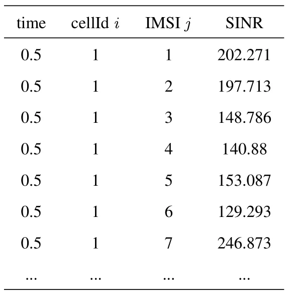
Table 3. Trace of SINR.

As exhibited in the table,the trace file mainly contains four key parameters.The simulation running time in seconds represents the simulation situation between the base station and the user node at that moment.CellId is the cell number of the collected data.International Mobile Subscriber Identity (IMSI) is an identification code that is used to distinguish different users in a cellular network and is not repeated in all cellular networks.The SINR value reflects the linearaverage of all resource blocks (RB) between the ith base station and the jth user node.In order to collect valid SINR data and make the positioning model accurate,a threshold value will be set for the collected SINR value.We reserve the data where the SINR value exceeds the threshold value.For those values below the threshold,it will be artificially modified to 0.

At the same time,based on the selected actual area,we use the building module of NS-3 platform to build buildings.Building construction takes into account the height of the floor,the size of the floor plan and the construction materials,because these are the factors that affect the signal transmission.

NS-3 contains three kinds of fadingtrace,namely Extended Pedestrian A model (EPA),Extended Vehicular A model (EVA) and Extended Typical Urban model (ETU).Considering the diversity of user node types,we mainly considered the EPA and EVA scenarios,and their moving speeds are 3 kmph and 60 kmph respectively.As shown in Figure 5,we have selected the change graph of SINR value under different scenarios and different numbers of user nodes.It is a simulation result of a unified two dimensional value grid,which represents the strongest SINR signal value of the base station at each point in the down link under different conditions.

4.2 Training Experiment of Positioning Model

Figure 5a shows the distribution of SINR values without considering scene fading.It changes linearly with the distance from the base station.In the case of adding the fading trajectory,considering the interference of the user equipment to the received and transmitted signals,the value of SINR will not decrease fixedly as the distance increases,but will show irregular changes with time and location.Therefore,the signal scene of Figure 5a is no longer considered,which has no reference for the prediction of the regional position.

Combined with the content of the Section III,we considered a neural network model with three hidden layers.The input data is a four dimensional matrix of SINR values containing four base stations.After three layers of hidden layer training with 10 neurons in each layer,the output is a nine dimensional matrix containing nine location regions.We use random 80 percent of the collected data as the training set,and the remaining 20 percent as the test set.It is set that when the accuracy of the test set prediction exceeds 90 percent,the training of the neural network is stopped,and a regional positioning model based on SINR is obtained.Collect the data of the new user node in the simulation platform again,and use these data as the verification set.The performance is measured by comparing the predicted user node location with the corresponding value of the validation set data.We consider the mean square error for performance measurement.The following equations give the definitions:

where Stestis the amount of data in the validation set,t(i)is the location of the ith user node predicted by the neural network regional positioning model,and y0(i)is the actual location of the ith user node.

After the training of the neural network training model is completed,we use the simulation platform to regenerate a large amount of data to verify the model.The result is shown in Figure 6.

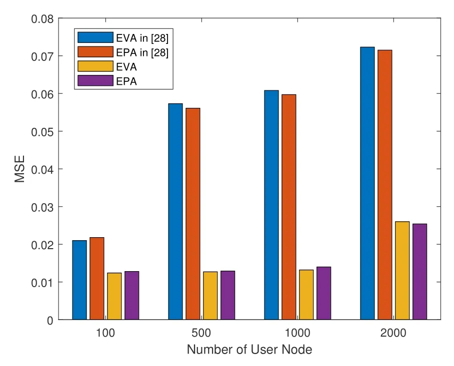
Figure 6. The relationship between MSE and user nodes in EVA and EPA scenarios.

As can be seen from Figure 6,compared with the result of[28],our experimental results have a greater improvement.This is due to the different divided areas and the different number of base stations selected for positioning.In[28],a hexagon is equally divided into 6 areas with the same area.The closer to the center,the closer the user node receives the SINR value from each base station,which will cause a prediction error.In this research,we divided the selected network scenario into 9 less crowded areas.The user node receives the SINR value from each base station to have a better discrimination,so the prediction effect will be better.From the results in Figure 6,it can be found that under the two channel fading trace,the results of position prediction are similar.This shows that the training model has good adaptability to the environment,and the change of the environment has little effect on the prediction of regional positioning.When the number of user nodes increases in the network environment,its prediction performance will decrease.This is because the interference signal in the network increases with the increase in the number of users,which leads to larger prediction errors.

4.3 Introduction of Edge Computing Node Deployment Framework

The main goal of this section is to output the ranking of potential edge computing nodes in order to minimize costs by choosing the best deployment location.The optimized deployment framework of edge computing nodes is shown in Figure 7.We determine the specific parameters of the area generated by SUMO and establish a coordinate system according to the simulation requirements.At the beginning of the simulation,the delay threshold,potential node deployment location,data transmission delay,number of edge computing nodes,computing resources,and user node requirements are limited.In order to adapt our framework to the need of cellular IoT,we modify the LTE module in NS-3 and adjust the parameters according to the 5G technical requirements and currently determined technologies.

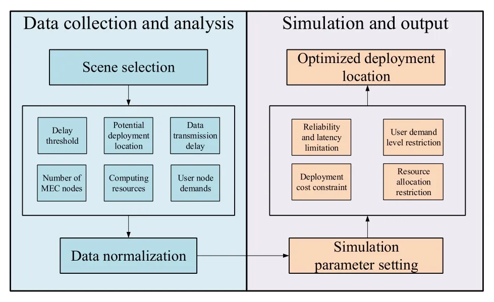
Figure 7. Framework for deploying edge computing nodes based on simulated annealing.

The simulation of the optimized deployment of edge computing nodes has mainly gone through two stages of data collection and analysis as well as simulation and output.

In the data collection and analysis stage,the collected data is normalized to meet the need of subsequent simulations.The SceneSelection module builds models of buildings and roads on the map to simulate real world interference,and generates user nodes to simulate demand distribution and user demand levels.In the next module,we will collect data by categories to divide the area of interest.Through the area positioning algorithm,the number of edge computing servers is determined to obtain the distribution of user data hot spots in the service area.When the demand is distributed in a large area with fewer user nodes,it is further optimized by analyzing key information such as the delay threshold and data transmission delay.Check whether there is a user node that needs service in each service area,and determine whether an edge computing node is to be deployed in this area.This stage allows us to simplify the areas where the number of users does not reach the service threshold,deploy a small number of edge computing nodes in these areas,or connect to edge computing nodes in other service areas,so the operating costs and deployment costs can be reduced.When data collection is completed,the normalized processing module is used to meet the simulation requirements of the next stage.

In the simulation and output stage,the optimization problem of edge computing node deployment is NPhard.Therefore,based on the SA method proposed by the predecessors,it was selected as the solution because it can list the desired results and has the applicability to solve the deployment of edge computing nodes.This is because the Metropolis criterion of the SA algorithm allows to accept a certain degraded solution,which is to accept a non-optimal solution with a certain probability.The Metropolis criterion is the key to the SA algorithm converging to the global optimal solution.And the Metropolis criterion accepts the degraded solution with a certain probability,so that the algorithm jumps from the local optimal trap.The acceptance probability Pais

where f(Sn) is the optimization result of the deployment cost of edge computing nodes after the nth iteration,T is the temperature during the current optimization process,and rand is a randomly generated random number in the (0,1) interval.Snis accepted as the new current solution when the acceptance probability value is greater than rand,otherwise the current solution Sn−1is retained.After introducing new key constraints,it is necessary to model a new problem of a more comprehensive cost function and obtain a method to solve the cost problem.After obtaining the deployment location of the edge computing node according to this method,it is necessary to check whether each location where the edge computing node is deployed is suitable.In addition,the analysis of user node locations and the differences in service levels bring additional complexity to the solution.

V.ANALYSIS OF SIMULATION RESULTS

In this section,we evaluated the performance of the algorithm under simulated real-world conditions to verify that the framework introduced in Section IV has applicability and usability in actual scenarios.

The SA method has been run and implemented to evaluate the performance of the relationship between the deployment cost of edge computing nodes and the number of user nodes.In (10),the transmission delay parameters of d(i,j)and LMare estimated based on the Euclidean distance between the user node and the edge computing node.The processing delay is obtained from the trace file obtained after NS-3 simulation.The simulation increases the number of user nodes from 100 to 500,and adds 100 users at a time.In the algorithm,the initial temperature is set to 10000,the minimum temperature is set to t,and the number of internal Monte Carlo cycle iterations is set to 100.It can be perturbed by multiple iterations,and multiple experimental simulations are performed before the temperature decreases.At the same time,the rate of change of each temperature is set to 0.95.In order to calculate the cost of the solution,the cost parameter is analyzed based on a common measurement unit after normalizing the data,so that any number of cost units is assumed to be equivalent to one capacity unit.The effectiveness of the numerical results was verified by running the algorithm multiple times.In addition,the solution cost,running time,and number of users of the optimal solution found by each method are estimated by periodically increasing the number of edge computing nodes (determined by the threshold of the positioning algorithm).The results are shown from Figure 8 to Figure 11.

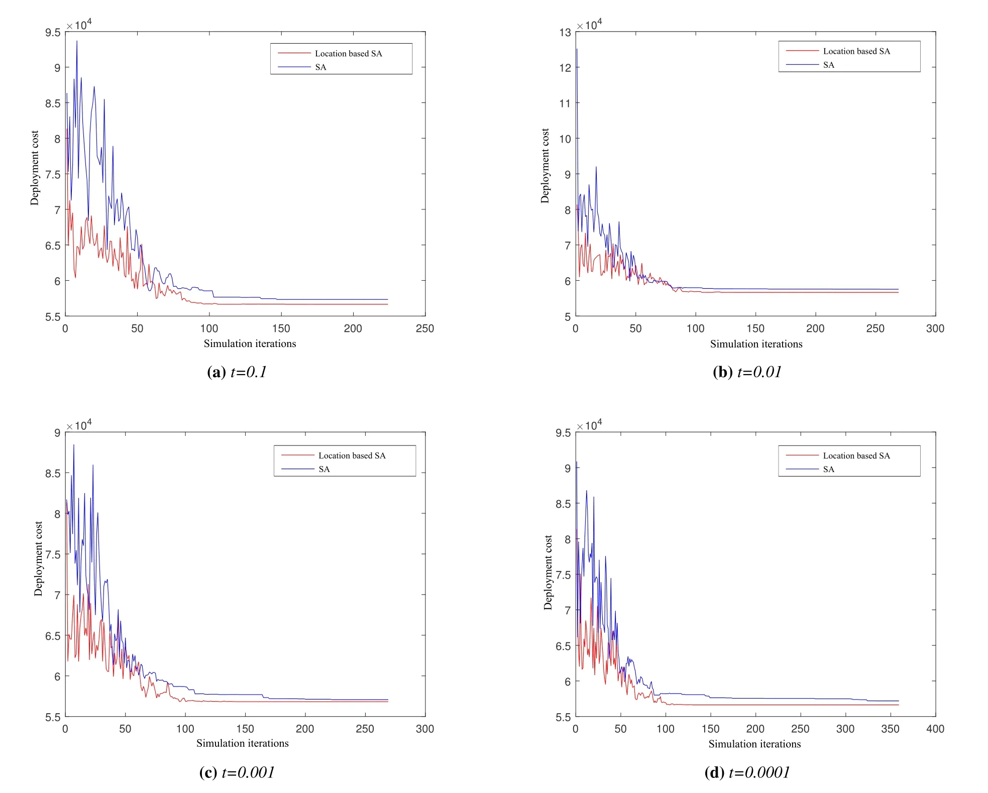
Figure 8. Deployment cost at different temperatures.

As displayed in Figure 8,in Figure 8a,when the stop temperature of SA is set to 0.1,the performance of the traditional SA is not as good as that of SA based on the data hotspot area proposed in this paper.From Figure 8a to Figure 8d,as the stopping temperature of SA decreases,the performance of the traditional SA can approach the algorithm we proposed.At the same time,the algorithm we proposed can converge faster and find the optimal deployment location of edge computing nodes faster.As the temperature decreases,the optimization results gradually stabilize,as shown in Figure 8d,when the temperature reaches 0.0001,the optimization results will appear smooth in the later iteration process.However,the traditional SA algorithm needs more iterations to gradually approach the results of our proposed algorithm.Therefore,compared with the traditional SA algorithm,the SA algorithm based on user data hotspot area can save a lot of computing time and has better optimization effect.

Figure 9a and Figure 9b display the simulation results when β is 20 and 30.The edge computing nodes in the figure are deployed in the optimized position according to the optimization algorithm,and the surrounding user nodes (red nodes) are connected to the corresponding edge computing nodes.The biggest difference is the number of edge computing nodes,which is caused by the different thresholds of the number of user nodes in the area.When the threshold of the number of user nodes is small,it means that the demand for edge computing nodes in this area is greater,and more edge computing nodes will be deployed.At the same time,the simulation time will be different.More detailed results are illustrated in Figure 10 and Figure 11.

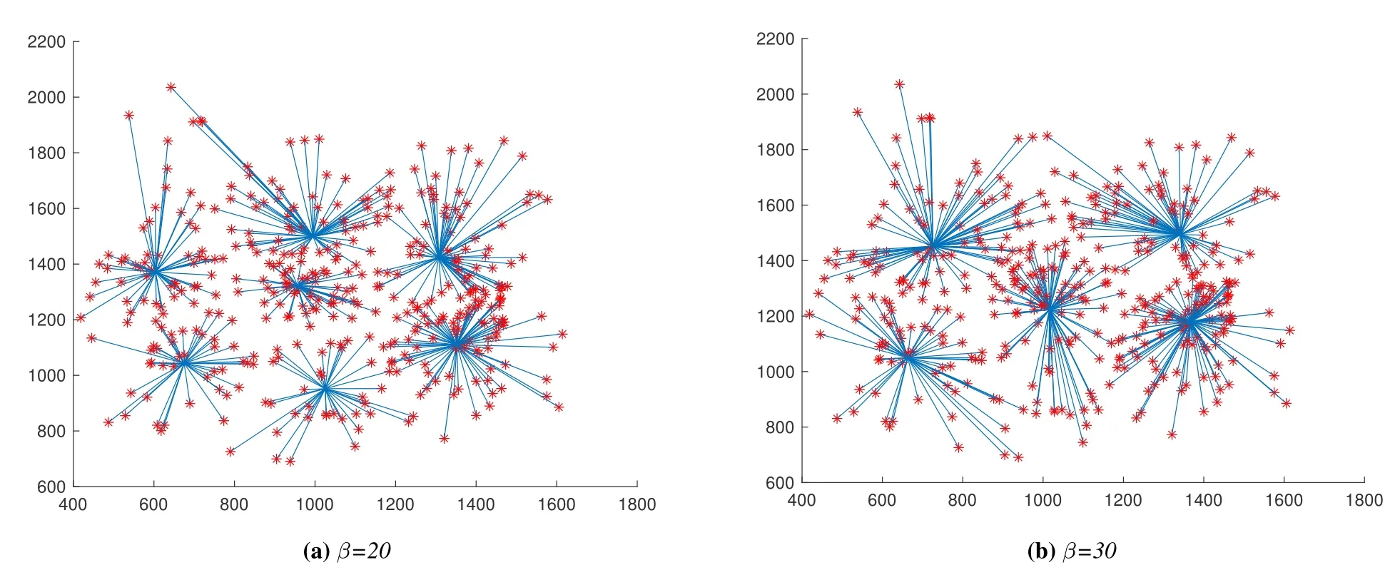
Figure 9. Simulation results under different thresholds.

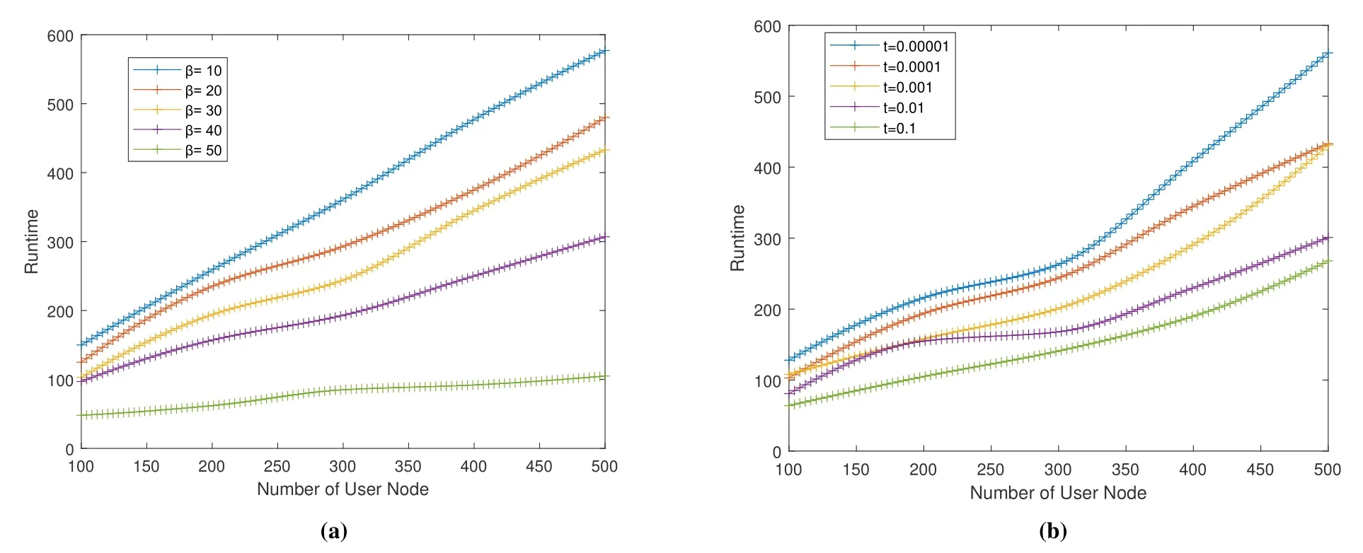
Figure 10. Simulation run time.

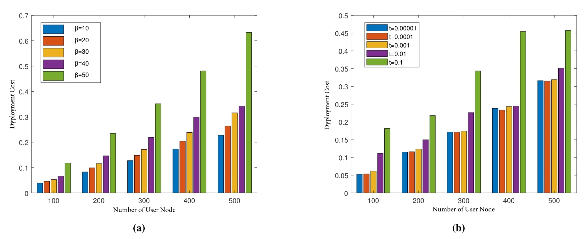
Figure 11. Edge computing node deployment costs.

Figure 10 depicts how the simulation run time changes as the number of user nodes increases under different conditions.In Figure 10a,the temperature of the SA method is set to 0.0001,and five trends are plotted in the interval from 10 to 50 thresholds.From the figure,we can see that regardless of the threshold,the running time of the simulation shows an upward trend as the number of user nodes increases.The reason is that the increase in the number of user nodes makes the algorithm more difficult.When the number of user nodes is the same,the simulation running time will decrease with the increase of the threshold.As the threshold becomes larger,it means that the certain area needs more users to deploy edge computing nodes,resulting in a reduction in the number of edge computing nodes.From the trend of the five lines in the figure,it can be seen that although the threshold is 50,the running time is the least,but it may cause too few edge computing nodes to provide the proper services,which ends the simulation early.Therefore,when the threshold is 40 or 30,under the condition of completing the task,the running time is less.With reference to Figure 11a,when the threshold is 30,the deployment cost of edge computing nodes is relatively more stable,and is lower than the threshold of 40.Therefore,it is more appropriate to set the threshold to 30.Figure 10b shows the change in simulation run time as the number of user nodes increases at different end temperatures.From the figure,we can see that when the number of user nodes is less than 300,the increment of the simulation running time is gentler,and then the lower the temperature,the greater the change in running time.Combined with the analysis of the deployment cost of the edge computing node in Figure 11b,under the condition that the deployment cost of the edge computing node is lower,the simulation effect is better when t=0.001.

The conclusion that can be drawn from these analyses is that the SA method has thoroughly explored the deployment space of edge computing nodes based on the determined minimum temperature 0.0001 and the temperature drop gradient value.The future work on this issue is how to reduce the execution time while not affecting the optimal parameter value of the algorithm performance.

VI.CONCLUSION

This paper has presented an optimized deployment scheme based on SA to solve the problem of deploying edge computing nodes in 5G networks under strict technical requirements.An experimental simulation platform has been established by combining NS-3 and SUMO to simulate the communication data in the actual scene.The use of a neural network-based regional positioning algorithm has greatly improved the positioning performance to reduce the complexity of edge computing node deployment.Based on the established simulation platform with actual environmental impact,the collected data is optimized to test the performance of the edge computing node deployment framework.Simulation results show that the performance of the proposed method under different parameters,and verify the advancement compared with the traditional SA method.The proposed method can show good performance in a variety of business types and can be used in real high-traffic hotspot scenarios.

ACKNOWLEDGEMENT

This work was supported in part by the Beijing Natural Science Foundation under Grant L201011,in part by the National Natural Science Foundation of China (U2001213 and 61971191),and in part by National Key Research and Development Project(2020YFB1807204).