Performance assessment of borehole arrangements for the design of rectangular shallow foundation systems

Marin Chwała,Danko J.Jerez,Hetor A.Jensen,Mihael Beer,d,e

a Wrocław University of Science and Technology,Poland

b Institute for Risk and Reliability,Leibniz University Hannover,Germany

c Departamento de Obras Civiles,Universidad Técnica Federico Santa María,Chile

d International Joint Research Center for Resilient Infrastructure&International Joint Research Center for Engineering Reliability and Stochastic Mechanics,Tongji University,Shanghai,200092,China

e Institute for Risk and Uncertainty and School of Engineering,University of Liverpool,United Kingdom

Keywords:Foundations Geotechnical engineering Bearing capacity Optimal borehole placement Soil spatial variability

ABSTRACT This study proposes a framework to evaluate the performance of borehole arrangements for the design of rectangular shallow foundation systems under spatially variable soil conditions.Performance measures are introduced to quantify,for a fixed foundation layout and given soil sounding locations,the variability level of the foundation system bearing capacities in terms of their mean values and standard deviations.To estimate these measures,the recently proposed random failure mechanism method(RFMM)has been adopted and extended to consider any arrangement of rectangular foundations and boreholes.Hence,three-dimensional bearing capacity estimation under spatially variable soil can be efficiently performed.Several numerical examples are presented to illustrate the applicability of the proposed framework,including diverse foundation arrangements and different soil correlation structures.Overall,the proposed framework represents a potentially useful tool to support the design of geotechnical site investigation programs,especially in situations where very limited prior knowledge about the soil properties is available.

1.Introduction

The growing interest in uncertainty quantification in geotechnical engineering observed in recent years (Chwała et al.,2022) is accelerated by the need to account for the considerable uncertainties arising in the estimation of natural soil parameters.In this regard,methods to handle these uncertainties have been developed not only from a general perspective (Cao and Wang,2013;Baecher,2017;Ching et al.,2018;Ching and Phoon,2020),but also to assess specific geotechnical systems such as foundations(Fenton and Griffiths,2005;Halder and Chakraborty,2019;Wu et al.,2020;Li et al.,2021;Wang et al.,2022),slopes(Huang et al.,2013;Javankhoshdel et al.,2017;Chen et al.,2020;Zhang et al.,2022),and retaining walls (Bathurst et al.,2019;Kawa et al.,2021).Despite the rapid development of probabilistic approaches in geotechnical engineering,as a recent report for the TC304 Time Capsule Project (Ching,2022) indicates,there are major gaps between the state of the art and state of the practice related to uncertainty quantification in geotechnical engineering.One of the mentioned gaps is between theory and practice.While engineers seek straightforward techniques,easy-to-implement methods,or results that can be directly used in practice,recent research developments in this area usually prove mathematically convoluted and difficult to implement.This highlights the need for methods that provide practical elements for decision making under uncertainty in geotechnical engineering applications.

One of the most important aspects of recent research in geotechnical engineering pertains to the development of optimal sampling schemes for site investigation.In this context,some reported approaches aim to reduce the error in soil strength parameter estimation (e.g.Goldsworthy et al.,2007a;Gong et al.,2017;Huang et al.,2020;Crisp et al.,2021;Guan et al.,2022).In general,the main goal of these methods is to maximize the robustness of site investigation programs while minimizing site investigation costs.Alternatively,application-specific approaches have been developed for the assessment of,e.g.foundation settlement (Goldsworthy et al.,2007b),slope stability (Jiang et al.,2020;Li et al.,2016a,2016b,2019),or pile foundations (Crisp et al.,2020).However,relatively little attention has been given to evaluate the impact of soil sounding locations on shallow foundation bearing capacity under spatially variable soil properties.Even though some approaches to estimate the bearing capacity of this class of systems have been reported(Al-Bittar et al.,2018;Kawa and Puła,2020;Bolaños and Hurtado,2021;Li et al.,2021),the effect of soil soundings has not been usually incorporated in their formulation.In this regard,the study by Li et al.(2022) assesses the effect of soil soundings on the reliability of an isolated shallow foundation using the random finite element method.Alternatively,the approach presented in(Chwała,2020b,2021)addresses bearing capacity estimation for cases involving a single rectangular foundation and up to two boreholes.Nevertheless,methods to assess the impact of multiple sampling locations on the bearing capacity of multiple foundations have not been yet reported.

It is the objective of this contribution to develop a framework to assess the performance of borehole arrangements for the design of rectangular shallow foundation systems.Four performance measures are proposed in terms of the standard deviations and mean values of the bearing capacities of the system.Since the estimation of these quantities using direct finite element-based techniques for spatially variable soil can be computationally very demanding or even prohibitive in real-life cases,a recently proposed approach named random failure mechanism method(RFMM) (Chwała,2019) is adopted and suitably extended to consider any number of foundations and boreholes,provided that the corresponding footings are sufficiently distant from each other.In this manner,efficient estimation of three-dimensional undrained bearing capacity considering spatially variable soil is enabled.Furthermore,the formulation is suitable for cases where very limited prior information about the soil is available.Overall,the proposed framework represents a potentially useful tool to identify optimal configurations of soil soundings and aid practical decision-making processes in the context of geotechnical site investigation programs.

2.Background

2.1.Spatially variable soil

Due to the heterogeneity of natural soils (e.g.Phoon,2017;Konkol et al.,2019),their inherent spatial variability (Phoon and Kulhawy,1999;Pieczyńska-Kozłowska et al.,2021),and the unavoidable errors arising in their monitoring processes (Yang et al.,2022),the consideration of uncertainties in the mechanical properties of soils is an important aspect of geotechnical engineering.In this regard,it is commonly accepted to model soil spatial variability by means of random fields (Fenton and Griffiths,2008),and this approach is used in this work.In particular,undrained soil conditions are considered in this contribution.The undrained shear strength,cu,is modeled as a stationary three-dimensional random field with a given correlation structure.Thus,the foundation bearing capacities become random variables.In this regard,their corresponding mean values and standard deviations are of particular interest in this work.It is noted that estimating such quantities can be numerically demanding,as it usually involves uncertainty propagation through complex nonlinear and large-scale threedimensional finite element models (e.g.Kawa and Puła,2020;Li et al.,2021).

2.2.Borehole placement for foundation design

Borehole placement can have a significant effect on the quality of information for geotechnical engineering analyses.Further,optimal sounding locations depend on the specific type of geotechnical structure under consideration (Goldsworthy et al.,2007b).This study addresses soil sounding placement for a fixed foundation layout,which is a common scenario in civil engineering.Boreholes are incorporated into the analysis by correlating the undrained shear strength along vertical lines at their locations with the rest of the soil domain (Chwała,2020b).This consideration tends to reduce,in general,the variability of the bearing capacity of the different foundations.While finding optimal borehole locations for a single foundation is conceptually simple,it is not straightforward for systems with multiple foundations.Thus,measures to enable the comparison between alternative soil sounding configurations for cases with multiple footings are proposed in the next section.It is noted that the adopted strategy is different from the implementation of conditional random fields(e.g.Li et al.,2016b;c,2019).

3.Performance measures for optimal borehole placement

Four measures are presented to compare the performance of alternative borehole locations for the design of shallow foundation systems.These measures rely on the mean values and standard deviations of the bearing capacities of the different foundations.It is noted that the choice of a proper performance measure is problem-specific,and it can depend on several factors such as,e.g.design requirements or the type of supported structure.In this context,alternative performance measures requiring only the mean value and standard deviation of the bearing capacities can be also implemented within the proposed framework.

To describe the scenarios considered in this work,nBboreholes andnFfoundations are considered.For a given borehole arrangement,the bearing capacity(p)of thekth foundation(k=1，…，nF),has mean valueμp，k,standard deviationσp，kand coefficient of variation vp，k=σp，k/μp，k,which are estimated by means of direct Monte Carlo simulation.

3.1.Average coefficient of variation

The arithmetic average of vp，knormalized by the coefficient of variation of the undrained shear strength,vcu,can serve as a measure of performance for a given borehole arrangement,which is given by

where the normalization by vcuis only for convenience.The measure can be useful to address cases in which all foundations are regarded as equally relevant,and the expected variability level across all bearing capacities is the primary element for decision making.

3.2.Maximum coefficient of variation

Instead of using the average coefficient of variation given in Eq.(1),the maximum coefficient of variation corresponding to the different bearing capacities can be a target for engineers as

This measure ensures that the coefficient of variation of the bearing capacity will be at mostψvvcufor all foundations.Such a formulation is convenient,for instance,when all foundations are regarded as equally important for structural safety and the designer’s intention is to ensure an upper bound for the variability level,in terms of the coefficient of variation,of all bearing capacities.

3.3.Average normalized variability measures

The measures defined in Eqs.(1)and(2)consider the variability levels of all bearing capacities,in terms of the coefficients of variation,as equally important.However,an optimal borehole configuration according to these two measures may not provide an optimal usage of the information retrieved by the available soil soundings.A convenient approach to address this issue is to consider measures that quantify the impact of boreholes in terms of the level of information gain;(e.g.Li et al.,2016b,2019).One way to achieve this is to compare the variability levels of the different bearing capacities in the cases with and without boreholes.In this regard,a measure called‘average normalized standard deviation’is proposed as

3.4.Maximum normalized variability measures

Based on the concept of usage of information,two alternative performance measures are defined in terms of the unconditioned and conditioned standard deviations and mean values of the different bearing capacities.The first is referred to as ‘maximum normalized standard deviation’,and it is given by

whereas the second performance measure is called ‘maximum normalized coefficient of variation’,and it is defined as

The previous measures quantify the maximum variability level,expressed as a percentage of the unconditioned standard deviations of coefficients of variations,of the system bearing capacities for a given borehole arrangement.Thus,such measures can be particularly useful to identify borehole locations in case the designer needs to ensure a minimum level of information usage for all foundations and,in addition,all foundations are regarded as equally important.

4.Numerical implementation

The evaluation of the measures proposed in the previous section entails,in principle,a relatively large number of Monte Carlo realizations of the bearing capacities to estimate their mean values and standard deviations.For three-dimensional cases involving multiple foundations,such as the ones considered in this contribution,the use of finite element models usually requires significant computational efforts to evaluate a single realization of the bearing capacities(Kawa and Puła,2020;Li et al.,2021).Moreover,finding an optimal arrangement of soil soundings would require,in principle,the nested evaluation of mean values and standard deviations within an optimization procedure.To circumvent these issues,an alternative approach is considered in this contribution.

4.1.Random failure mechanism method (RFMM)

The RFMM(Puła and Chwała,2018;Chwała,2019)is adopted to estimate the bearing capacity of rectangular footings for spatially variable soil.The method is based on applying the spatial averaging technique (Vanmarcke,1983) to dissipation regions resulting from the kinematical approach of limit analysis based on the upper bound theorem (Chen,1975;Pietruszczak,2010).The idea is to generate spatially averaged soil parameters in the dissipation regions instead of using the original random field together with a finite element model of the entire soil domain,which significantly improves numerical efficiency.Specifically,the RFMM is based on the discretization of the original random field to a correlated set of random variables that characterize the mechanical properties of interest.The correlation between them is determined by a covariance matrix,which depends on both the geometry of the failure mechanism and the random field parameters.This formulation avoids the need for explicit realizations of the entire random field associated with large-scale three-dimensional finite element models or computationally expensive reanalysis of such models.Overall,the RFMM provides significant computational savings for bearing capacity estimation under spatially variable soil conditions(Chwała,2020a).For completeness,a short review of the most important features of the method is provided below.

The failure geometry of a representative rough foundation base consists of 30 dissipation regions,as shown in Fig.1.For reference purposes,all types of dissipation regions and their short names are as follows.The rectangular dissipation regions are ABFE,DCHG,AMEP,NORS with corresponding short namest1,t2,t3,t4;the triangular regions are ABI,ICD,EFW,GWH,TAM,TON,UEP,USR,IAJ,TAJ,IKL,TKL,WEZ,WXY,UEZ,UXY with corresponding short namest5,…,t20;the cylindrical regions are ABC-EFG,AMN-EPR with corresponding short namest21andt22;and the conical regions are EFG-W,ABC-I,EPR-U,AMN-T,AKJ-I,AKJ-T,EYZ-W,EYZ-U with corresponding short namest23,…,t30.Formulas for the estimation of the bearing capacity associated with this failure mechanism are provided in Appendix A.

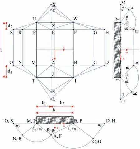
Fig.1.Failure geometry for undrained bearing capacity of a rectangular foundation.

Once the optimal failure geometry corresponding to the expected value of undrained shear strength is found,the Vanmarcke spatial averaging technique(Vanmarcke,1983)is applied to obtain a so-called moving average field.This process averages the random field within each dissipation regiont.Finally,as previously mentioned,the initial random field of undrained shear strengthCuis discretized to a set of correlated single random variablesCu，ti,i=1，…，30.Thus,each random variable is assigned to one dissipation region.Since the random field under consideration is stationary,the mean value ofCu，tiis preserved.On the other hand,the variance is reduced by the so-called variance functionγ（t）.The covariance between two single random variables is given by

wheretiandtjare the considered dissipation regions,|·| is the Lebesgue measure of the corresponding region(in this case area or volume),andRis a covariance function.In this study,two types of correlation structures are considered.The first corresponds to the Gaussian covariance function:

The second to the Markovian covariance function:

whereθx，θyandθzare the scales of fluctuation(SoF)in thex，yandzdirections,respectively,and Δx,Δyand Δzare the lag distances along the corresponding axes.Detailed derivations for the variance and covariance formulas can be found in(Chwała,2019).Then,the 30-by-30 covariance matrix describing the correlation between the random variables corresponding to the 30 dissipation regions is given by

Note that in casei=j,a variance is obtained.

4.2.Extension to multiple foundations

To preserve the correlation between all dissipation regions,the covariance matrix from Eq.(10) must be expanded to include information on the correlation between all dissipation regions occurring in thenFfoundations.For each foundationFk(k=1，…，nF) the corresponding covariance matrix is determined as

wherek=1，…，nF.Note that the covariance matrices and dissipation regions for the different foundations are indexed by the foundation numberk.

Eq.(11) characterizes the correlation between the random variables associated with a single foundation.However,it is also necessary to quantify the correlation between the random variables of different foundations.To this end,new formulas have been derived.As an illustration,the covariance between the random variables associated with the ABC-EFG cylinders of foundationskandl(see Fig.2) for a Gaussian covariance function is given by

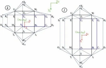
Fig.2.Failure geometries of two rectangular foundations for evaluating the covariance between the dissipation regions of two failure mechanisms.

whereωx=Note that the previous expression represents a 6th-order integral expressed in a global coordinate system,which is evaluated using a Monte Carlo integration scheme(Chwała,2019).For illustration purposes,Fig.3 presents the parametrization scheme considered in the formulation of Eq.(12).An analogous formula can be obtained for the Markovian covariance function in Eq.(9).

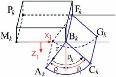
Fig.3.Parametrization of dissipation region AkBkCk-EkFkGk.

The covariance matrix[C]k，lcomprises the covariances between the random variables associated with regionskandl,wherek，l=1，…，nF.Note that in casek=l,the covariance matrix of Eq.(11)is obtained.Specifically,the covariance matrix [C]k，lis given by

Once the covariances between all random variables involved in the problem are obtained,an enlarged covariance matrix of size 30nF×30nFis generated.This matrix can be readily used to estimate the mean values and standard deviations of the bearing capacities of the different foundations.However,such a matrix refers to the unconditional case,i.e.,no information about the boreholes has been yet included.To address this issue,an approach to include multiple boreholes in bearing capacity assessment is implemented in this contribution.

4.3.Extension to multiple boreholes

The enlarged covariance matrix described in the previous section is further extended to consider cases with multiple boreholes.To this end,the geometry of each borehole is first assumed as a straight vertical line.Then,the mean value of the undrained shear strength along that line is assumed to be the mean value of the stationary random field.Further,a small variability ofcuat the borehole location is assumed to reflect measurement accuracy.Based on this formulation,the properties of thenBrandom variables associated with thenBboreholes can be obtained following the same principles described in the previous subsections.FornB≥2,the covariances between all possible pairs of boreholes need to be determined.For a Gaussian correlation structure,the covariance between boreholesbiandbjis given by

where (xbi,ybi) and (xbj,ybj) are thexandycoordinates of theith andjth borehole expressed in a global coordinate system.Additionally,the covariances between the random variables of the different boreholes and all failure regions need to be determined.As an example,the covariance between boreholebi,i=1，…，nBand the cylinder portionAkBkCk-EkFkGk,k=1，…，nFfor a Gaussian correlation structure is given by

The extension of the covariance matrix in Eq.(13)is obtained by adding as many rows and columns as the number of boreholesnB,which leads to a final covariance matrixof size (30nF+nB) ×(30nF+nB).In addition,the assumptionθx=θyis adopted in this study.Hence,θx=θy=θhandθz=θvare considered for the horizontal and vertical SoF,respectively.Finally,it is noted that all covariance matrix terms are positive in the present formulation.Therefore,special strategies to treat negatively correlated parameters are not required by the proposed framework.

4.4.Summary of the proposed procedure

4.5.Remarks

In accordance with previous studies (e.g.Fenton and Griffiths,2008),a lognormal stationary random field is used to model the undrained shear strength of the soil.Then,the computation of the covariance matrix,,requires specifying the sizes and locations of the different foundations as well as the borehole positions.Generally,the algorithm detailed in Appendix B can be used for any location and number of boreholes,and any size and number of rectangular foundations.Further,this procedure can be repeated for alternative borehole arrangements to compare their performance.In this regard,it is noted that only the covariances associated with the borehole locations must be updated for alternative soil sounding configurations,whereas the covariances between dissipation regions must be determined only once for a given foundation arrangement.This feature is advantageous from a practical viewpoint.While this contribution focuses on stationary random fields,it is noted that the same basic approach can also be applied,in principle,to non-stationary cases (Chwała and Kawa,2021).Finally,the only restriction of this approach is that the different foundations must be sufficiently separated in order to ensure that the failure mechanisms are not interfering with each other.Such a minimum distance can be taken as two times the foundation width(e.g.Gourvenec et al.,2006;Alzabeebee,2022).In practice,this assumption implies that mechanical interaction between different footings cannot be explicitly evaluated within the proposed framework.

5.Examples

Three examples involving systems with multiple foundations are presented to illustrate the capabilities and applicability of the proposed approach.Example 1 illustrates the effect of the number of Monte Carlo simulations and the number of boreholes in a relatively simple foundation system.In Example 2,a symmetric foundation layout is addressed to study the effect of the scales of fluctuation and correlation function type on the proposed performance measures.Finally,Example 3 considers a non-symmetrical arrangement of foundations of different sizes to show the applicability of the proposed framework to identify optimal regions for borehole placement.

5.1.Example 1

The example concerns three square footings (width of 1 m)separated 10 m from each other.These are shown in Fig.4 with their corresponding indices.For illustration purposes,the undrained shear strength(cu)is modeled as a lognormal random field with Gaussian correlation structure,mean value of 100 kPa,and standard deviation equal to 50 kPa.

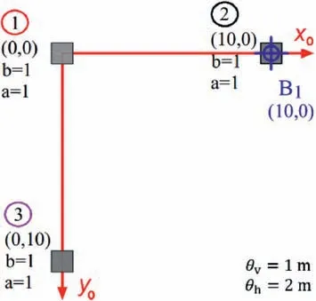
Fig.4.Placement of square footings and a single soil sounding.

First,a scenario with a single borehole located directly under the second footing is considered with an anisotropic correlation structure given byθv=1 m andθh=2 m.The mean values,standard deviations,and coefficients of variation of the bearing capacities of the different footings,in terms of the number of samples,NMCS,are presented in Fig.5.From the figure,it is seen that placing the borehole directly under the center of a foundation results in a significant reduction of the variability of its bearing capacity,which is reasonable from an engineering viewpoint.In addition,the results indicate that a few hundred samples (in the order of 100-300) are adequate to obtain sufficiently accurate estimates of the different quantities under consideration.

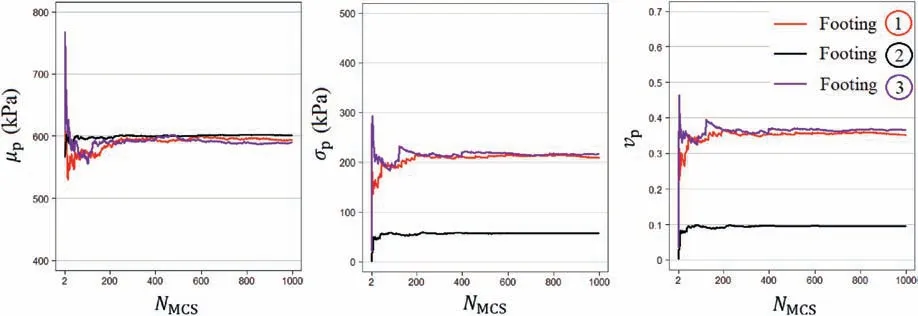
Fig.5.Evolution of mean values,standard deviations,and coefficients of variation of the bearing capacities in terms of the number of samples for a single borehole.

A case considering two boreholes,as shown in Fig.6,is studied next.Note that one of the boreholes is located in the vicinity of footing 1,whereas the other soil sounding is placed equidistant from footings 1 and 3.To illustrate the effect of the horizontal SoF,two values ofθhare considered,namely,θh=2 m(scenario 1)andθh=10 m (scenario 2).Hence,scenario 1 entails a weaker correlation of the undrained shear strength than scenario 2.In both scenarios,the vertical SoF is taken asθv=1 m.The corresponding results are shown in Fig.7.Several observations can be made from the figure.First,the values ofσp，1and vp，1are the lowest in both scenarios.This is expected since the boreholes are located closer to footing 1.Second,these values are significantly smaller in scenario 2.For this case,a higher correlation in the undrained soil strength enhances the beneficial effect of the soil soundings on footing 1,which ultimately reduces the variability of the corresponding bearing capacity to a greater extent.Third,the opposite effect is observed forσp，2and vp，2,andσp，3and vp，3remain almost equal in both scenarios.This suggests that the variability reduction achieved by the presence of soil soundings tends to decrease when they are located farther from the foundations.Finally,it is seen that scenario 1 provides smaller expected values of the bearing capacity than scenario 2 for all footings.In other words,a stronger correlation is associated with a reduced bearing capacity for this configuration of footings and boreholes.This can be interpreted as a manifestation of the worst-case effect (Cami et al.,2020;Li et al.,2022;Pieczyńska-Kozłowska et al.,2022),i.e.the expected value of the bearing capacity achieves its minimum for finite values of the fluctuation scales.In general,this minimum is observed for values of the horizontal fluctuation scales that are comparable to the foundation width (Cami et al.,2020).

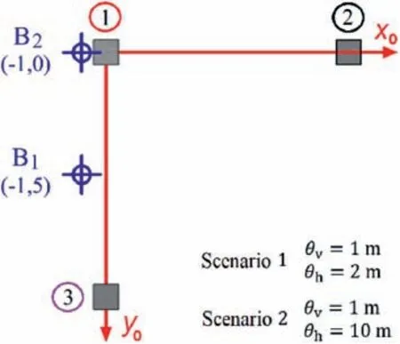
Fig.6.Placement of square footings and two soil soundings.

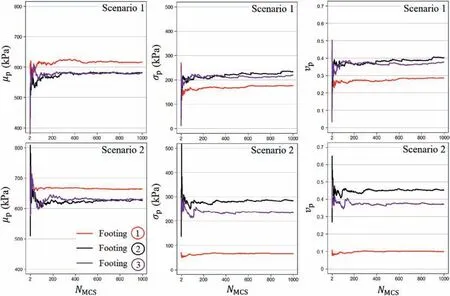
Fig.7.Evolution of mean values,standard deviations,and coefficients of variation of the bearing capacities in terms of the number of samples for two boreholes and two alternative correlation structures.

5.2.Example 2

This example considers a symmetric foundation system of four identical square footings with each side of 1 m.In addition,the random field adopted to characterize the undrained shear strength is the same considered in Example 1.

Numerical results in the context of this example suggest that,in general,the vertical fluctuation scale has a very limited impact on the normalized performance measures defined in Eq.(3)-(6).To illustrate this,Fig.8 presents the contours ofandobtained for a single borehole in the casesθv=0.4 m andθv=1 m,with the horizontal SoF kept constant for both cases asθh=10 m.It is noted that the performance measures are considered as explicit functions of the coordinates（x，y）of the borehole under consideration,i.e.=（x，y）and=（x，y）.To obtain these contours,the performance measures are evaluated for a number of alternative borehole locations.Specifically,the coordinates for the borehole are associated with a regular grid with a step of 1 m along each direction.From the figure,it is seen that the contours ofare practically overlapping for both values ofθv(see Fig.8a and b),and analogous results can be observed for(see Fig.8c and d).Furthermore,additional validation calculations indicate that the same behavior is observed when considering alternative values for the horizontal SoF.Thus,even thoughθvdoes have an impact on the standard deviation of the bearing capacities (e.g.Fenton and Griffiths,2008;Chwała,2019),the normalized measures show a very weak dependence on this parameter for this example.

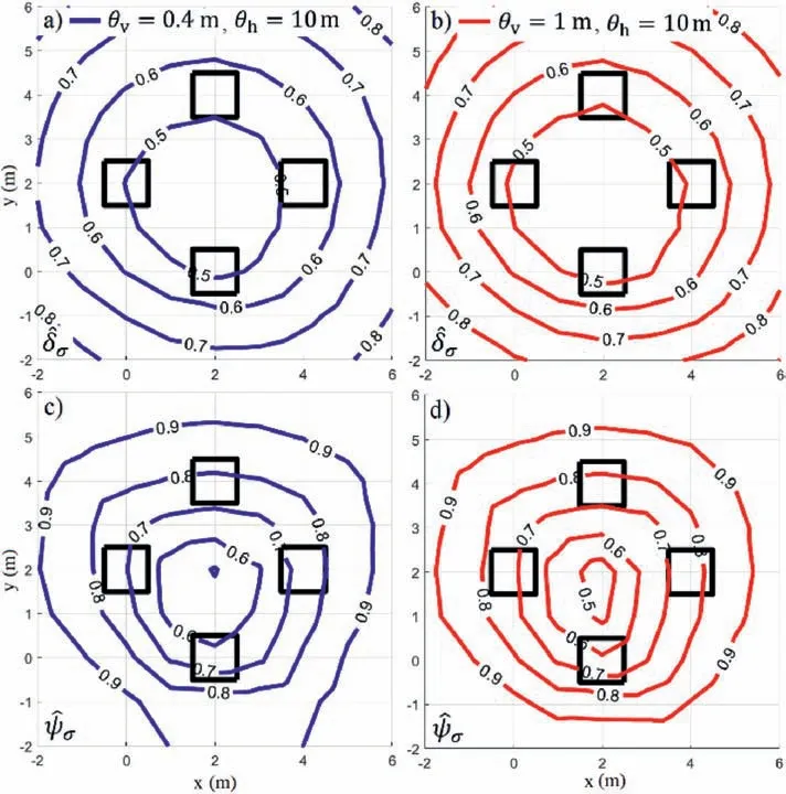
Fig.8.Contours of normalized performance measures for θh=10 m and different vertical SoF: (a) ,θv=0.4 m,(b) ,θv=1.0 m,(c),θv=0.4 m,and (d),θv=1 m.

The results shown in Fig.8 are associated withθh=10 m,which leads to a relatively strong correlation between the bearing capacities of all foundations.As a result,both measures present a similar behavior with respect to the borehole position for this case.In fact,the optimal locations identified by both performance measures lie near the geometrical center of the foundation system.These results agree with those obtained for settlements of square footings,in which sampling in the center of the footing system is found to be beneficial when no centralized footing exists(Goldsworthy et al.,2007b).However,for shorter horizontal fluctuation scales,there are some differences between these measures.This is illustrated in Fig.9,where the contours ofandare shown forθh=4 m.Four local minima are observed for,which indicates that local information gain becomes more important for this measure in cases with relatively mild correlation.On the other hand,the optimal location identified byis at the center of the foundation system,which agrees with the results observed in Fig.8.In addition,it is noted that the values ofare close to one in the entire domain (i.e.,the function is practically constant over the entire domain).Further,additional calculations indicate thatis almost constant forθh＜4 m and,therefore,a unique optimal borehole location cannot be identified in such cases.Meanwhile,forθh＞4 m the most convenient region for placing the borehole is consistently observed at the center of the foundation system.In other words,a weak dependence of the optimal borehole location is observed whenis adopted as performance measure for scenarios involving relatively strong horizontal correlation.This is particularly relevant when considering how challenging in engineering practice is the determination ofθh(e.g.Ching et al.,2018).If no prior information about the site of interest is available,it is recommended to consider fluctuation scales from studies of sites with similar geological history (e.g.Pieczyńska-Kozłowska et al.,2017) or,if such data are not accessible,reference values reported in the literature (e.g.Cami et al.,2020).

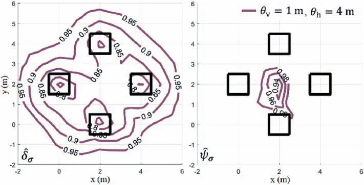
Fig.9.Contours of (left) and (right) for θv=1 m and θh=4 m.

For illustration purposes,a case involving two boreholes is now considered.One borehole is located under the center of the leftmost footing,whereas the second borehole can be placed at any desired position.Fig.10 shows the contours ofandobtained for different locations of the second borehole.In this case,the performance measures are considered as explicit functions of the coordinates（x，y）of the second borehole,while the first borehole is kept fixed at the positionx=0 m,y=2 m.It is seen that the optimal regions for the second borehole location are relatively similar for both performance measures,i.e.,they are adjacent to the rightmost foundation.Nonetheless,the shapes of both contours are slightly different,with ︿ψσbeing less sensitive to the position of the second borehole.This agrees with the results observed in Fig.9,in the sense thatis more sensitive to local usage of information than.Finally,it is noted that these optimal locations are conditional on a fixed borehole location and,thus,they are most likely sub-optimal from a global perspective.This highlights the need of extending this framework to assist optimal decision-making processes for geotechnical site investigation programs involving multiple soil soundings.

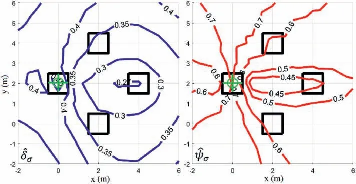
Fig.10.Contours of (left) and (right) for two boreholes with θh=10 m and θv=1 m.The first borehole is fixed at x=0 and y=2.

In the previous scenarios,a Gaussian covariance function has been considered.To illustrate the effect of the correlation structure,Fig.11 presents the contours ofobtained for Gaussian and Markovian covariance functions.Two scenarios in terms of the horizontal SoF are considered,namely,θh=2 m andθh=10 m.From the figure,it is observed that changing the type of covariance function does not affect the optimal region for borehole placement in this case.This is an important insight because the covariance functions are generally assumed and are quite difficult to determine based on available data (e.g.Ching et al.,2019).Note that both correlation functions are commonly used in modelling soil spatial variability in geotechnical engineering,but their properties are relatively different.From the comparison of Eqs.(8) and (9),it is seen that the Gaussian covariance function provides stronger(weaker)correlation for distances shorter(longer)than 2θ/π when compared to the Markovian covariance function.As a result,the contours shown in Fig.11 for the Gaussian and Markovian cases show differences in the values offorθh=10 m.Meanwhile,such differences are significantly smaller forθh=2 m,as expected.

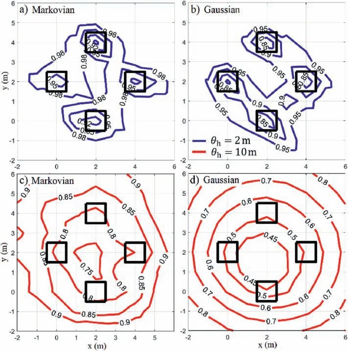
Fig.11.Contours of obtained for θv=1 m and different correlation cases: (a) θh=2 m,Markovian,(b) θh=2 m,Gaussian,(c) θh=10 m,Markovian,and (d) θh=10 m,Gaussian.

5.3.Example 3

The previous examples consider foundation arrangements with some symmetry axes,for which optimal borehole locations can be regarded as more intuitive.However,the proposed framework can be most beneficial in cases involving general foundation layouts for which convenient locations for the soil soundings are difficult to identify a priori.In this example,a nonsymmetrical foundation arrangement of four footings with different dimensions is studied in order to show the capabilities and applicability of the approach.For illustration purposes,the random field of the undrained shear strength is the same considered in Example 1,a Gaussian correlation structure is assumed,and the vertical SoF is taken asθv=1 m.

First,to study the effect of the horizontal SoF,Fig.12 presents the contours of the performance measureforθh=4 m,θh=10 m,andθh=20 m.As in Example 2,the performance measures are considered as explicit functions of the borehole coordinates（x，y）.In general,the results are qualitatively similar to those reported in the previous examples,that is,tends to prioritize local information gain when shorter correlation scales are considered.In fact,local minima appear in all foundation centers forθh=4 m,and the corresponding global minima seem to be located under the smallest footings.On the other hand,the contours associated with longer fluctuation scales,i.e.θh=10 m andθh=20 m,show a different behavior.In these cases,the most convenient borehole locations seem to lie near the left and central footings.Finally,it is noted that the optimal regions identified in all cases are not straightforward to determine based on engineering judgment only.This highlights the usefulness of the proposed framework,as it can provide non-trivial insight for decision-making purposes.

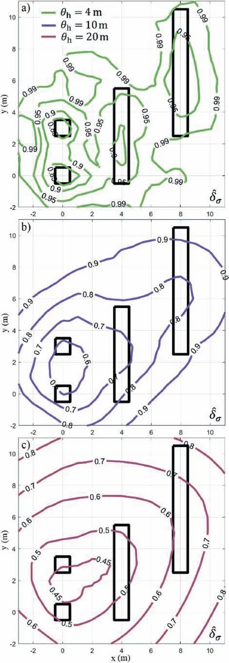
Fig.12.Contours of for different horizontal SoFs:(a)θh=4 m,(b)θh=10 m,and(c) θh=20 m.

The previous results correspond to the average normalized standard deviation,i.e..To illustrate the effect of choosing an alternative performance measure,the contours corresponding toforθh=4 m,θh=10 m,andθh=20 m are presented in Fig.13.Note that these results are significantly different from those presented in Fig.12.For the caseθh=4 m,it is found that≈1 in the entire domain.Thus,from a practical viewpoint,it seems that no optimal region can be identified in this case.This indicates that,in this example,a single borehole cannot reduce the variability level of all foundations if the undrained shear strength of the soil is weakly correlated.On the other hand,for longer scales of fluctuation the optimum locations seem to lie closer to the centroid of the foundation system whenis considered as performance measure.This behavior agrees with the results presented in the previous example,in the sense thattends to assign more importance to global information gain rather than local variability reduction.

To illustrate the differences between the four types of measures introduced in this work,the contours of,,δvandψv,associated with the location of a single borehole,are compared in Fig.14 forθh=6 m.Recall thatδvandψvconsider only the variability levels conditional on a given borehole arrangement,whereasandadditionally incorporate the unconditional variability measures as normalizing constants.From the figure,it is seen that the differences between the contours of the average-based measures,i.e.andδv,are quite small.On the other hand,the results obtained forandψvdiffer significantly.Not only the global minima are attained at different locations,but also the shapes of the corresponding contours are dissimilar.Moreover,is approximately equal to one in the entire domain,which agrees with the behavior observed in Fig.13a.Such a situation can indicate,for instance,that more boreholes may be needed to reduce the uncertainty of bearing capacities.Thus,this measure can be potentially useful to decide on the appropriate number of soil soundings to implement in a given geotechnical site.

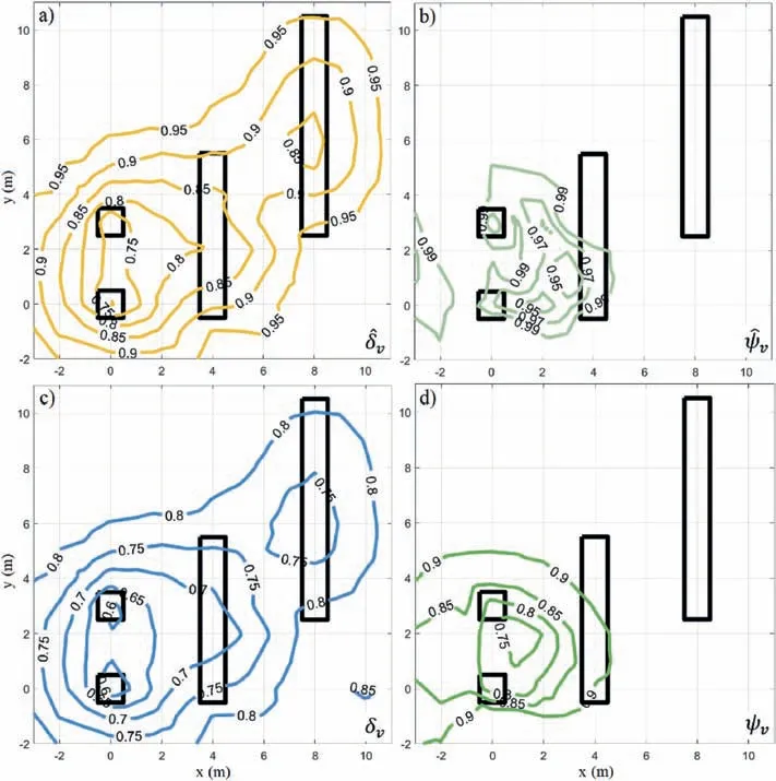
Fig.14.Contours of different performance measures for θh=6 m: (a),(b),(c) δv,and (d) ψv.

Fig.15 shows the contours of the four performance measures forθh=20m.In this case,which involves a higher value for the horizontal SoF,the differences betweenandδvare negligible.Similarly,the contours ofresemble those ofψv.These results are reasonable from the engineering viewpoint and agree with those reported in the previous example since,for a given borehole location,the coefficients of variation of the different foundations tend to be more similar between each other when a stronger correlation is taken into account.

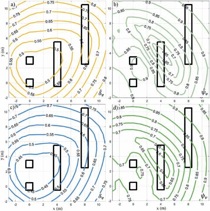
Fig.15.Contours of different performance measures for θh=20 m: (a) ,(b),(c) δv,and (d) ψv.

Finally,the comparison of Fig.12c with Fig.15a indicates that the contours in both plots are very similar between each other.Since the only difference between the performance measuresandis that the latter also incorporates the mean values in its definition,this suggests that the effect of bearing capacity mean values on the optimal borehole location is minor for this case.Moreover,additional validation calculations in the context of this example indicate that analogous results are obtained for different scales of fluctuations,which seems reasonable from an engineering viewpoint.

6.Conclusions

This contribution has presented a framework to assess the performance of soil sounding configurations for the design of rectangular shallow foundation systems.Four performance measures are proposed in terms of the mean values and standard deviations of the bearing capacities of the different foundations.To estimate these quantities,the RFMM is extended to consider any arrangement of rectangular foundations and boreholes for a class of shallow foundation systems in which the corresponding footings are sufficiently distant from each other.In this manner,computationally intensive approaches based on,e.g.finite element models are circumvented and,simultaneously,three-dimensional soil variability is rigorously incorporated into the analysis.

Three examples involving different foundation arrangements and soil correlation characteristics have been addressed to evaluate the capabilities of the proposed framework.Based on the corresponding numerical results,the following conclusions can be drawn:

(1) Measures based on the maximum operator tend to give more importance to global information gain,whereas those based on the average operator prioritize local usage of the information provided by the borehole array.

(2) Based on the assumptions of the approach,the effect of the vertical fluctuation scale on the behavior of the normalized performance measures seems to be negligible for all the examples considered in this work.

(3) For different performance measures,the Markovian and Gaussian correlation functions provide similar optimal borehole locations in the examples presented in this work.This insight can be important for future applications.

(4) Sufficiently accurate estimates of the performance measures can be obtained with a few hundred samples(in the order of 100-300),which can be advantageous from a practical viewpoint.

Based on the previous discussion,the proposed approach provides valuable insight about the performance of different borehole configurations for the design of shallow foundation systems.In general,the choice of a particular performance measure is problem-specific and depends on several factors,such as project requirements and the nature of supported structures.However,alternative performance measures can be directly implemented within the proposed framework as long as the mean values and standard deviations of the foundation bearing capacities are involved in their definition.Overall,the approach presented in this contribution constitutes a flexible,numerically efficient,and potentially useful tool to assist the design of geotechnical site investigation programs with explicit uncertainty treatment.

Future research efforts aim to extend the proposed framework to optimal borehole placement when multiple soil soundings are available and to decide whether the assumed number of boreholes is sufficient or not.In this case,an appropriate optimization strategy is needed.Another research direction involves the treatment of situations with multiple foundations that are very close to each other.This entails,in principle,the explicit inclusion of mechanical interaction between different footings.Additional subjects for future research include the treatment of scenarios involving sequential construction of footings,the inclusion of trends for undrained shear strength,and the extension of the methodology to systems with non-rectangular foundations.Some of these topics are currently under consideration.

Data availability statement

Some or all data,models,or code that support the findings of this study are available from the corresponding author upon reasonable request.

Declaration of competing interest

The authors declare that they have no known competing financial interests or personal relationships that could have appeared to influence the work reported in this paper.

Acknowledgments

The first author would like to thank for the support of the Polish National Agency for Academic Exchange under the Bekker NAWA Programme (Grant No.BPN/BEK/2021/1/00068),which founded the postdoctoral fellowship at the Institute of Risk and Reliability at Leibniz University Hannover.The first author would also like to thank to Prof.Wengang Zhang and Chongzhi Wu (School of Civil Engineering,Chongqing University) for inspiring discussions initiated by High-end Foreign Expert Introduction program (Grant No.DL2021165001L) by the Ministry of Science and Technology(MOST),China.The second author would like to thank the support from ANID(National Agency for Research and Development,Chile)and DAAD (German Academic Exchange Service,Germany) under CONICYT-PFCHA/Doctorado Acuerdo Bilateral DAAD Becas Chile/2018-62180007.The third author gratefully acknowledges the support by ANID under its program FONDECYT (Grant No.1200087).

Appendix A.Supplementary data

Supplementary data to this article can be found online at https://doi.org/10.1016/j.jrmge.2023.05.009.