Angular disturbance prediction for countermeasure launcher in active protection system of moving armored vehicle based on an ensemble learning method

Chun-ming Li , Gung-hui Wng ,*, Hi-ping Song , Xu-feng Hung , Qi Zhou

a China North Vehicle Research Institute, Beijing,100072, China

b School of Aerospace Engineering, Huazhong Univerisity of Science and Technology, Wuhan, 430074, China

Keywords:Active protection system Angular disturbance prediction Deep ensemble learning

ABSTRACT The active protection system (APS), usually installed on the turret of armored vehicles, can significantly improve the vehicles’survivability on the battlefield by launching countermeasure munitions to actively intercept incoming threats. However, uncertainty over the launch angle of the countermeasure is increased due to angular disturbances when the off-road armored vehicle is moving over rough terrain.Therefore, accurate and comprehensive angular disturbance prediction is essential to the real-time monitoring of the countermeasure launch angle. In this paper, a deep ensemble learning (DEL)-based approach is proposed to predict the angular disturbances of the countermeasure launcher in the APS based on previous time-series information. In view of the intricate temporal attribute of angular disturbance prediction, the sampling information of historical time series measured by an inertial navigation device is adopted as the input of the developed DEL model.Then,the recursive multi-step(RMS)prediction strategy and multi-output (MO) prediction strategy are combined with the DEL model to perform the final angular disturbance prediction for the countermeasure launcher in the APS of a moving armored vehicle. The proposed DEL model is validated by using the different datasets from real experiments.The results reveal that this approach can be used to accurately predict angular disturbances,with the maximum absolute error of each DOF less than 0.1°.

1. Introduction

An active protection system (APS) is designed to prevent the armored vehicle against anti-vehicle threats by launching countermeasure munitions to intercept the incoming threats, such as anti-tank missiles or projectiles,which can effectively enhance the survivability of vehicles on the battlefield [1]. The APS controller can dynamically calculate the coordinate of the intersection point of the incoming target's trajectory and the countermeasure's straight flight line at the radius of its protection sphere, and then control the countermeasure launcher fixedly mounted on the vehicle turret. The launcher will respond to the launch angle command and fire a countermeasure toward the intersection point.Finally, the target will be intercepted by the detonation of the countermeasure. Some APS products, such as Trophy mounted on Israel MK4 Merkava Main Battle Tank(MBT)and US M1A2 Abrams MBT, and Iron Fist on Dutch CV90 infantry fighting vehicles have been developed. To reduce the response time, the APS controller sends the launch angle command only once. Upon receiving the command, the countermeasure launcher executes the command immediately. But due to the six-degrees-of-freedom (6DOF) disturbances to the launcher generated by the off-road vehicle moving over rough terrain,the countermeasure may miss the target if these disturbances are not considered. Therefore, it is necessary to predict the values of these disturbances at the moment of the launching of the countermeasure for the APS controller to adjust the launch angle.

Unfortunately, it is challenging to accurately predict the disturbances for several reasons: 1) Moving armored vehicle is affected by driver manipulation and the complex terrain; 2) The complicated disturbances are composed of vibrations caused by rough terrain and vibrations generated by high power diesel engine,transmission system,suspension system,etc.;3)It is difficult to evaluate and quantify road surface characteristics; and 4) The disturbance frequency range to be predicted is wide and complex.To improve prediction performance,various studies on time series prediction and trajectory analysis have been conducted. Han et al.[2] developed a predictive control framework based on a neural network model and adaptive learning algorithm to predict the dynamic behavior of nonlinear systems. Similarly, an improved artificial neural network(ANN)based on the radial basis function is proposed to identify adaptive modulation formats [3]. Zhang et al.[4] presented an adaptive neural control algorithm using the multiport event-triggered scheme,which can predict the sail force compensation according to the information of heading angle and wind direction. And in time series prediction, conventional Bayesian filtering methods are widely used,such as Kalman[5]and extended Kalman filters [6]. However, these methods have poor long-term time series prediction performance and cannot be used to well analyze intricate vehicle movements. To address these problems, more complex models with good performance, such as dynamic Bayesian networks (DBNs) [7], Gaussian mixture models[8], and Gaussian process models [6,7], have been developed.Specifically, using DBNs, a framework for more flexible trajectory analysis can be realized, in which graphical models are adopted to describe the different critical factors that govern vehicle trajectories,and the relation between these critical factors can be learned from input data. In this context, DBNs can be employed to effectively predict the trajectory and vibration time series explicitly by modeling of physical processes. Nonetheless, the model structure determined by prior knowledge is not adequate to capture different kinds of real dynamic scenes.It is also not appropriate to use DBNs for real-time prediction due to their inefficient inference steps.Different from the conventional methods, in deep learning (DL)methods, a deep neural network driven by massive data (i.e., a data-driven method)is used to find the physical and mathematical relationship between time series data.The existing DL methods for sequence prediction are basically divided into three types [9],namely, convolutional neural networks (CNNs), recurrent neural networks (RNNs), and other models (e.g., graph-based approaches or combined approaches). Gated RNNs, including long short-term memory (LSTM) [10] and gated recurrent units (GRUs) [11], are widely used in sequence data prediction. Srivastava et al. [12]established a fully connected LSTM (FC-LSTM) model with an encoder-decoder structure and multi-step prediction strategy,which can be used to simultaneously rebuild the input data and predict future time-series data.Inspired by FC-LSTM,Shi et al.[13]presented a prediction model named ConvLSTM for end-to-end precipitation now casting, which used multiple convolution and LSTM layers to perform state-to-state or input-to-state changeover.An encoder-decoder approach [14], which used multiple LSTMs to analyze patterns in past trajectories and generate sequences of future trajectories, was developed for trajectory prediction in a sequence-to-sequence manner. Sergio et al. [15] put forward a novel architecture to simultaneously handle the rasterized map and the data from the LiDAR. In this approach, two-branch CNNs were used as backbone to extract the input features, and then three different neural networks were adopted to process the concatenated features for prediction of the vehicle trajectories.Li et al.[16]suggested a novel sequence prediction approach to predict the future flow parameters of supersonic cascades using bidirectional LSTM (BiLSTM) and a fully convolutional neural network (FCNN).Yan et al.[17]designed a CNN-LSTM-based approach for the multitime air quality forecasting, and when combined with a spatiotemporal clustering method, this approach exhibited better performance than the CNN-based method.Liu et al.[18]investigated a novel architecture named SCINet for time series forecasting,which used a sample convolution kernel and interaction for temporal modeling. However, the prediction accuracy and robustness of different algorithms for different degrees of freedom (DOFs) are inconsistent,which makes it difficult to accurately predict different DOFs with a single algorithm. And at present, there has been no research on the prediction of angular disturbances for the countermeasure launcher in APSs.

In this paper,a deep ensemble learning(DEL)-based approach is introduced to predict angular disturbances by using the competitive selection strategy to select the winning model from three models through the validation metrics, which improve the accuracy and robustness of multi DOFs prediction.First,an APS model is established considering the disturbance of the moving armored vehicle. Second, the sampling information of historical time series from the inertial navigation device is used to generate a measured real-world dataset. Then, this dataset is fed into the proposed DEL model to train each basic predictor.Finally,a competitive selection strategy is employed to select the predictor with the best validation accuracy to perform the final prediction of angular disturbances using test data.The primary contributions of this study are listed as follows:

(1) An innovative DEL model using LSTM, CNN-LSTM [17], and SCINet [18] is developed for time series prediction to improve the robustness and accuracy of multi-time prediction with the long-term dependency problem.

(2) A competitive selection strategy is proposed to adaptively select the basic predictor with the best validation accuracy of the ensemble model, which can improve the accuracy of angular disturbance prediction.

(3) A real-world dataset is constructed to validate the effectiveness of the proposed DEL method, which considers complex situations.

The rest of the paper is organized as follows. The model establishment process is introduced in Section 2. The details of the proposed DEL model are described in Section 3.Case analysis with experiment is presented in Section 4. Finally, the conclusion and future work are presented in Section 5.

2. Disturbance model establishment

The APS model in an armored vehicle is shown in Fig. 1. To realize the real-time detection of incoming targets in the airspace,the detection radars of the APS are arranged on the turret.Furthermore, a launcher is fixedly mounted on each side of the turret, and two countermeasure munitions can be deployed from each launcher. Since the detection radars are symmetrical on the turret,the origin of the radar coordinate system is set at the center point of these radars, as shown in Fig.1.

Fig.1. APS model in an armored vehicle.

The start time of one target interception process is set at the moment when the first data package about the incoming target found at the maximum distance is received from the detection radar,and meanwhile the radar coordinate system at this moment is set as the global coordinate system. Then the global coordinate system is fixed during this target interception solving procedure,while the radar coordinate system, turret, and countermeasure launcher move with the moving vehicle. The inertial navigation device mounted on the turret measures the angular disturbances and linear displacements of the launcher in real time.The detection radar outputs one frame of the target's trajectory data every 3 μs,covering the distance, speed, azimuth, pitch, and yaw angle of the target in the radar coordinate system.Each time the APS controller receives the target data, it will convert these data in the radar coordinate system into the data in the global coordinate system first.Next, the controller approximates the trajectory of the incoming target to a straight line and then tracks its trajectory.Therefore,the encounter moment TPtotalwhen the countermeasure hits the target can be derived from the incoming target's speed and the distance between the target and intersection point.

For a given turnover time Tturnof the launcher and flight time Tammunitionof the countermeasure before explosion, the launch angle command sending moment TPdecisionis calculated by TPdecision= TPtotal- Tturn- Tammunition. At the moment TPdecision,the APS controller finishes solving the coordinate of its intersection point and sends the countermeasure launch angle command. The goal of sending the command at TPdecisionis to ensure that the countermeasure is launched in the right direction at TPlaunchand reaches the intersection point at TPtotal. The flow diagram of the APS is shown in Fig. 2.

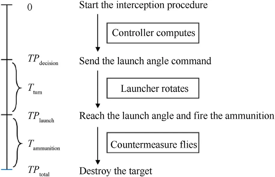
Fig. 2. Flow diagram of the active protection system (APS).

Because the launch angle command is sent at TPdecisionto the launcher without stabilization capability, it is necessary to predict the launch angular disturbance value at the countermeasure launch moment TPlaunchso as to adjust the command.

According to the linear displacement dx,dy,dzof the launcher at TPlauch, the intersection point P(xp,yp,zp) in the global coordinate system is given by

where Ai, Bi, Ci, and Di（i=1,2) are the fitting coefficients of the equation of the straight flight line of the incoming target trajectory at TPdecision.

Since the launchers and radars are all fixedly mounted on the turret, the launch angle should be calculated in the radar coordinate system at TPlaunch. After the interval Tturn, 6DOF disturbances dx,dy,dz,θx,θy,θzexist and should be taken into account.Thus the intersection point P(xp,yp,zp)is transferred into the coordinate P(xr,yr,zr) in the radar coordinate system,which is formulated as

where dx,dy,dzare linear displacements in the directions of the XYZ axes respectively,and θx,θy,θzare the angular disturbances around the XYZ axes directly measured by the inertial navigation device.As the linear acceleration of the armored vehicle is very small, the linear displacements dx,dy,dzare equal to the speed measured by the inertial navigation device multiplying the time Tturn.

Then according to the coordinate P(xr,yr,zr) and the launcher coordinate(xm,ym,mm)in the radar coordinate system,the launch angle can be deduced as follows.

where α and β indicate the azimuth and pitch angles respectively.Thus, predicting the angular disturbances θx,θy,θzis vitally important for determining the APS launch angle command.

3. Time series prediction method based on a deep ensemble model

In this section, an innovative DEL model is built for the prediction of the launch angular disturbance in the time domain based on LSTM, SCINet, and CNN-LSTM.First, each basic predictor is trained using the historical information of the time series. Then, diverse prediction strategies, including a recursive multi-step (RMS)strategy and a multi-output(MO)strategy,are integrated with the basic predictor to perform future prediction. Finally, a competitive selection strategy is used to select the most suitable predictor for the final prediction of the test data in each DOF.

3.1. Construction of the basic predictors

3.1.1. LSTM

RNNs, which is a natural generalization of artificial neural networks, have been widely adopted for sequence modeling. Recent studies have revealed that the two variants of gated RNNs,GRU and LSTM, can achieve better performance in regression and classification tasks. This section briefly introduces the RNN and LSTM.

The structure of a vanilla RNN is shown in Fig.3(a).Given input data X =（x1,x2,x3,…,xT) in the sequence, where T is the overall length of the input data,the current hidden state htof the RNN can be computed as follows:

Fig. 3. Architecture of RNN and LSTM.

where xtrepresents the current input symbol at time step t,f（•)is an activation function or a feedforward network,W is the input-tohidden weight,b is the bias of a single neuron,and U is the state-tostate recurrent weight. Notably, the current hidden state htis calculated by using both the current input information xtand the previous hidden state ht-1, which allows the RNN to effectively utilize the previous information to perform future prediction.

However, satisfactory performance cannot be achieved using RNNs when the input data have more long-term dependencies.To address this fundamental problem, several LSTM variants have been proposed by integrating forget gates and memory cells.Here,we follow the basic implementation of an LSTM. The basic LSTM architecture,as shown in Fig.3(b),consists of the input gate it,the output gate ot, the forget gate ktand the memory cell ct.Different from the RNN,in an LSTM,memory content in ctis first updated for further calculation of the current hidden state ht, which is computed as follows:

After the updating of memory content,the current hidden state htis computed as follows:

In the LSTM,the forget gates close and carry the information of memory cells across many time steps if their features are detected.In other words, long-term dependencies can be handled using the LSTM. In addition, the input gates are used to decide when to override or keep the information in the memory cells, and the output gates to control the error from different connections.In this context, LSTMs can be used to adaptively learn long-term dependencies to perform better predictions.

3.1.2. CNN-LSTM

Fig. 4 is a typical CNN structure, which uses local connections and shared weights to extract effective features from the original data by alternately stacking convolutional layers and pooling layers and finally outputs the extracted features by a fully connected layer.

Fig. 4. Basic structure of CNN.

(1) Convolutional (Conv)layer

In a CNN,the convolutional layer serves as the feature extraction layer, in which the convolution operation is performed for feature extraction from the original data and further highlight the original information representations. For example, the convolutional layer uses a 3 × 3 convolution kernel to slide horizontally on the input data in order to extract the corresponding feature map from the original data information.

The formula for the extraction of feature map m is defined below:

where w is the coefficient of weights,σ is the nonlinear activation function,k and l are the row and column of the convolution kernel sliding on the original data map each time, x is the data at the corresponding position, and b is the bias.

(2) Pooling layer

The pooling layer is also called the down-sampling layer,which is generally connected after the Conv layer,and the pooling process is a process of secondary extraction of data features.Conv layers can learn various data features with the combined action of multiple convolution kernels.Various pooling operations are used in a CNN,such as max pooling,average pooling,and spatial pyramid pooling.Take max pooling as an example:

The above formula describes the max pooling process,where m is the value of different features in the pooling window area. Assume an n-dimensional column vector. Max pooling is used to extract and retain the maximum value in m.After max pooling,the original data features n×n are compressed into redundant features of the data and thus are greatly reduced.This leads to a significant reduction of the input data of the next layer of the neural network.Therefore, the amount of calculation in the data dissemination process, training network overfitting and coincidence risk are reduced. To constitute the feature extraction layer in the CNN, the pooling layer is linked after the convolutional layer and they are alternately stacked.

(3) Fully connected (FC) layer

The FC layer generally appears after several Conv layers and pooling layers, which aims to integrate the local representations from the final pooling layer into a complete and dense feature vector. The full connection process is described by:

where y is the output data of the FC layer, w is the weight coefficient, b represents the bias, and σ represents the nonlinear activation function.

The overall architecture of a CNN-LSTM is shown in Fig. 5. As depicted in the figure, the one-dimensional CNN and LSTM are integrated to perform sequence prediction. The CNN is used to extract features so as to generate feature vectors and fully mine the information of time-series data from different angles. The LSTM takes features from the CNN as input and outputs the final prediction result.

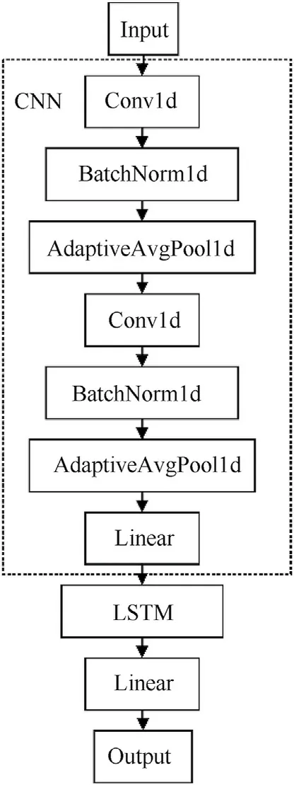
Fig. 5. The overall architecture of CNN-LSTM.

3.1.3. SCINet

SCINet is designed for time series prediction,which uses sample convolution and interaction networks. The overall structure of SCINet is depicted in Fig. 6. SCI-Block is the basic block in SCINet,and used to downsample the input features of data into two subsequences, as shown in Fig. 6(a). Then, different convolutional kernels are used to process each subsequence so as to extract both heterogeneous and homogeneous representations from the sequences. Additionally, interactive learning is employed between the two subsequences to compensate for the information loss during the downsampling process. As shown in Fig. 6(b), a binary tree structure using multiple SCI-Blocks is adopted to build the final SCINet. Notably, all low-resolution mechanisms are reshaped and concatenated into a new feature after the downsampling process;then,the new feature is added to the raw input for final prediction.To extract complex temporal features, a stacked SCINet using multiple SCINets and intermediate supervision can be constructed,as depicted in Fig. 6(c).

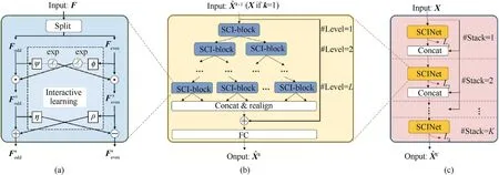
Fig. 6. The overall structure of SCINet [18]: (a) SCI-Block; (b) SCINet; (c) Stacked SCINet.

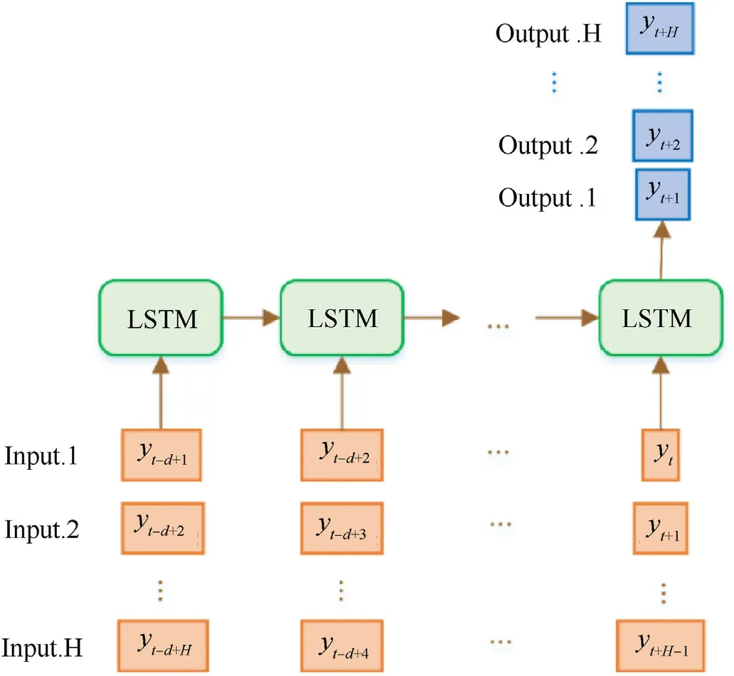
Fig. 7. Schematic diagram of the RMS prediction strategy.

3.2. Prediction strategies

According to the number of input variables,there are univariate time series prediction and multivariate time series prediction.Considering predicted future moments, there are single-step time series prediction and multi-step time series prediction. Compared with single-step prediction, multi-step time series prediction requires continuously predicting multiple time steps into the future based on historical observation data, which undoubtedly lead to increased complexity,error accumulation,decreased accuracy,and increased uncertainty.Jointly modeling the multi-step observations is the key to realizing continuous multi-step prediction as the continuous multi-step prediction data are not independent and identically distributed.

To build a multi-step prediction model, four strategies are commonly used, namely, the multioutput (MO) strategy, encoderdecoder strategy, direct multi-step strategy, and recursive multistep (RMS) strategy. Direct multi-step prediction aims to construct a model for each time point that needs to be predicted,which is cumbersome and time-consuming. In RMS prediction, a single-step prediction model must first be constructed and then the values of previous prediction steps are used to gradually generate predictions. In achieving multi-step prediction, the model is relatively simple and easy to train, but accumulated errors are inevitably introduced. The MO strategy is used to directly establish a multi-step prediction model but the relationship between the prediction sequences is not considered, so the overall prediction error at a low level cannot be guaranteed.In addition,it is not easy to optimize the multi-step model using an MO strategy due to the increased model complexity. In the encoder-decoder strategy, the input is first converted into a fixed-length tensor using an encoder.Then, this fixed-length tensor is decoded into the predicted sequence by the decoder considering the sequence dependencies between the predicted sequences.In this paper,the RMS prediction and MO prediction strategies are used for prediction, and when combined with the basic predictors mentioned in Sec. 0, they exhibit better performance. For brevity, an LSTM is used as an example to illustrate different prediction strategies.

3.2.1. RMS prediction strategy

The main component of RMS prediction is single-step prediction,and only one LSTM model needs to be constructed.To predict the sequence at the next moment, the prediction value of the previous moment is used as the input, and the output value of multi-step prediction is obtained by multiple iterations. Fig. 7 shows the schematic diagram of RMS prediction.

Fig. 8. Schematic diagram of the MO prediction strategy.

Given an input sequence with N samples [y1, y2, …, yN], the output sequence with K values[yN+1,…,yN+K]is predicted.A onestep ahead prediction model f（•)is trained,which is expressed by

The model f（•) is first adopted to predict the first-step value.Then,the predicted value is used as part of the input to the model f（•) to predict the next-step value. Finally, K values are predicted after multiple iterations.

Suppose the trained model is, and the predicted value can be expressed as

Its performance is degraded due to noise in the iterative process.If the dimension of the output sequence H exceeds the dimension d of the input sequence,then at some point in the prediction process,all inputs to the model will be predicted values rather than actual observations. Hence, the cumulative error of RMS forecasts is a potential factor in accuracy degradation.Despite these limitations,RMS strategies have been effectively used to predict real-time sequences using neural networks, like RNN and CNN.

3.2.2. MO prediction strategy

The MO prediction strategy is used to directly predict a vector whose length is the total quantity of points to be predicted. Fig. 8 shows the schematic diagram of the MO prediction strategy.

Given an input sequence with N samples [y1, y2, …, yN], the output sequence with H values[yN+1,…,yN+H]must be predicted.A time-series multi-output forecasting model F is trained, which is given by

where F is a vector-valued function and w∊RHis a noise vector.

Assuming that the trained model is︿F,the predicted value can be expressed as

The MO prediction strategy maintains the stochastic correlation between predicted values of the time series. Although the relationship between predicted series is not considered, it has been effectively used in numerous practical multi-step time series forecasting tasks.

3.3. Ensemble strategy

After each basic predictor is trained independently using training data from each DOF (i.e., univariate modeling), an ensemble strategy is used to combine them into one DEL model for further prediction.The essence of model integration is to integrate the output of multiple models by weighting. Therefore, the core goal is to determine the weight of each model in the DEL model.For a multi-model with m outputs, the outputs at time t can be expressed bythen the integrate output can be expressed as:

where ωi,tis the weight of the ith model at time t, and ︿yi,tis the predicted value of the ith model at time t. The most common ensemble learning strategy is the weighted average method, in which the average of the multi-model outputs is calculated as the final output. Using this method, the independent models in the multi-model strategy are treated equally. However, if any independent model performs poorly or unstably,the integration results will be significantly affected. Therefore, the weighted average method is sensitive, unstable and susceptible to outliers. Different from this method, in the performance-based integration strategy,corresponding weights are assigned to each independent model in the validation set on the basis of their performance and weighted integration is performed to the output results of multiple models.

Common performance-based integration strategies include the inverse root mean square error and competitive selection strategies. Here, the latter is selected as the ensemble strategy. The competitive selection strategy refers to the use of validation sets to select the prediction model outperforming others as the best model. The final output value by the multi-model strategy is determined by the output value of the best performing model.Therefore, the weight selection of the models in the competitive selection strategy can be expressed as

4. Case analysis with experiment

To verify the effectiveness of the developed DEL approach, the disturbance model in the real world that considers different complex situations is used as a case study in this section.

4.1. Dataset generation

To predict the launch angular disturbances, it is necessary to predict multiple steps in three DOFs, including the rotation angles of the X-axis,Y-axis,and Z-axis.These rotation angels are measured with a sampling rate of 333 Hz and detected by an XW-GI7690 inertial integrated navigation device [19] installed in the armored vehicle turret, as shown in Fig. 10. The total running time of the system is 13.38 s,which generates data of each DOF with a length of 4460.In addition,the predictor should predict at least 80 points in 240 ms to meet the minimum requirement of the time Tturn.

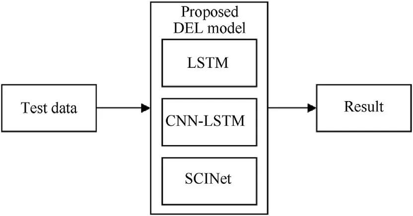
Fig. 9. The proposed DEL model.

Fig.10. Schematic diagram of Seq2Seq.

To speed up the training process and eliminate the effects of dimensional difference,all of the data were normalized to the range of [-1,1] by the following scaling equation:

where Xnormalis the normalized data, X is the original data.

Then we need to split the data of each DOF into a training set and testing set using the sliding window method. The ratio between the training and testing sets is 0.95:0.05. Since the models are trained in different ways,the data are generated differently.For the LSTM-MO, CNN-LSTM-MO, Seq2Seq, and SCINet models, each DOF is split using a 176-width sliding window with 1 step size.The first 96 points of each sample are the input, the last 80 points are the actual labels,and each variable i is cut to obtain a set of sliding window data segments, which can be formulated as

For LSTM-RMS and CNN-LSTM-RMS, each DOF is split using a 97-width sliding window with 1 step size. The first 96 points of each sample are the input, and the last 1 point is the actual label,

For Transformer, each DOF is split using a 96-width sliding window with 1 step size. The 96 points of each sample are the input, and real labels are generated by masking the 5 points after the input serial,

4.2. Experiment settings

The proposed method is compared with the autoregressive integrated moving average(ARIMA),Holt,Seq2Seq[20],transformer[21] and each basic predictor in Section 3.1 using different prediction strategies (i.e.,LSTM-RMS,LSTM-MO,CNN-LSTM-RMS,LSTMMO). In this case, Seq2Seq and Transformer are combined MO prediction strategies.The input size of all models is set to 96,while the output sizes of the model with the MO strategy and RMS strategy are set to 80 and 1, respectively.

4.2.1. Structural settings of the basic predictors

(1) Structural settings of the LSTM and CNN-LSTM methods

We fix the kernel size to 3 in all convolution layers, while the channels of the first and second convolution layers are fixed to 32 and 64.In addition,the sizes of the first and second pooling layers in the CNN-based model are set to(32,50)and(64,10).The neural numbers of the first and second linear layers (i.e., the fully connected layer) are set to 256 and 80. The 128-dimensional memory cells in the LSTM are used to better receive and comprehend the features from the last FC layer. Similarly, the number of memory cells for LSTMs used in LSTM-RMS and LSTM-MO is set to 128.

Fig.11. Measured data for the three DOFs: (a) Rotation angle of X-axis; (b) Rotation angle of Y-axis; (c) Rotation angle of Z-axis.

(2) Structural settings of Seq2Seq

The schematic diagram of Seq2Seq,as shown in Fig.11,consists of multiple LSTMs.In this paper,the encoder of Seq2Seq contains 10 LSTMs,and each LSTM is constructed with 16-dimensional memory cells. The decoder of Seq2Seq contains 80 LSTMs with 16-dimensional memory cells for each to perform the final prediction.

(3) Structural settings of Transformer and SCINet

For SCINet, the number of SCI-Blocks is set to 13, and the number of layers of the tree structure is set to 3. For Transformer,the number of multi-head attention in the encoder is set to 10,and the feature length of the encoder is set to 250.

(4) Structural settings of ARIMA and Holt

ARIMA and Hold model are two traditional time series prediction methods. For ARIMA, the parameters are searched within the constraints and selected to minimize the given index,and then the best ARIMA is fitted to the univariate time series. For Holt, the smoothing coefficients are automatically selected based on the time series data.

4.2.2. Training details and evaluation metrics

To adjust the loss function during the training process, the commonly used Adam optimizer[19] is adopted. The batch size of 32 and the initial learning rate(LR)of 3×10-4are selected as the hyperparameters of Adam. Additionally, an cosine annealing LR scheduler [22] is utilized to decay the LR for each batch, which is expressed as follows:

where ηtis the current LR, ηinitialis the initial LR, ηminis the minimum value of LR,Tmaxis the number of epochs in each restart,and Tcuris the number of current epochs.In this study,Tmaxand ηminare fixed at 50and 3× 10-6, respectively. In our experiments, the number of epochs is fixed at 500, which is sufficient for the convergence of the proposed method.

The maximum absolute error (MAE) and the root mean square error (RMSE) are employed as the metrics in this work. The MAE represents the local error, while the RMSE represents the global error. Each metric indicator is close to zero, indicating the better performance of the DEL model. The MAE and RMSE can be formulated as follows:

where yiandare the true and predicted responses at the ithtesting sample, and n is the number of testing samples.

5. Results and discussion

The performance comparison of univariate time-series prediction using the real-world measured dataset with three DOFs is shown in Table 1.From the table,it can be concluded that DEL is the ensemble model with the best validation MAE and RMSE in all cases, having superior performance over other basic methods.

Table 1 Performance comparison on the real-world dataset.

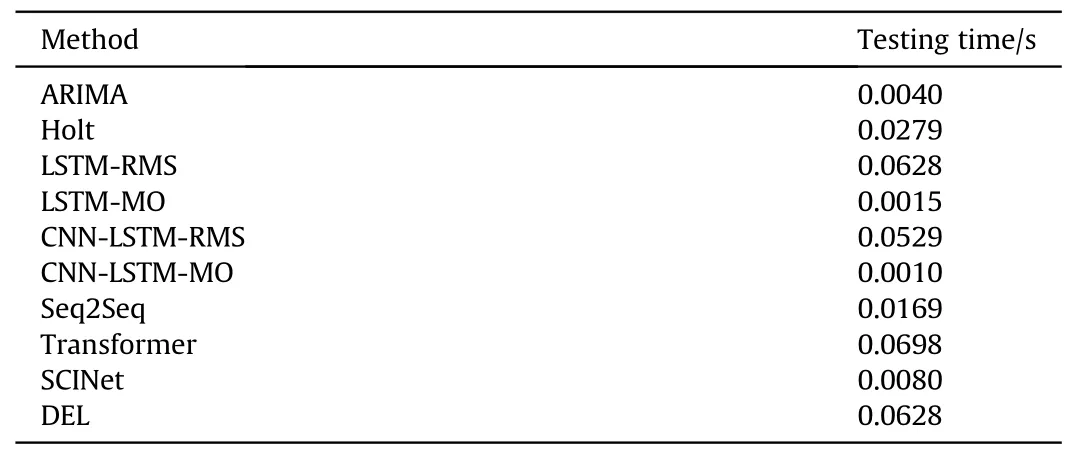
Table 2 Prediction time of different methods on the real-world dataset.

where V1,V2,V3 represent the rotation angles of X-axis,Y-axis,and Z-axis, respectively.

For V1 prediction (i.e., the rotation angle of X-axis), the SCINet approach has the best forecast performance with an MAE of 0.0308,while the Transformer approach exhibits the worst performance with an MAE of 0.2866.Fig.12 presents the best and worst results of the X-axis angular values on one testing sequence,which obviouslyillustrates the ability of SCINet to find the tendency of the time series in terms of the rotation angle of X-axis.

Fig.12. Prediction results about the rotation angle of X-axis of (a) SCINet and (b) Transformer.

Fig.13. Prediction results about the rotation angle of Y-axis of (a) SCINet and (b) CNN-LSTM-MO.

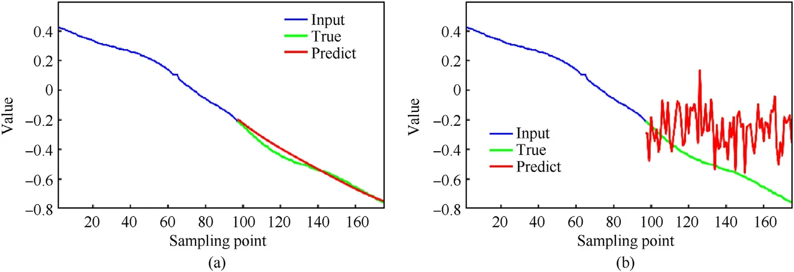
Fig.14. Prediction results about the rotation angle of Z-axis of (a) LSTM-RMS and (b) CNN-LSTM-MO.

For V2 prediction (i.e., the rotation angle of Y-axis), the SCINet approach has the best forecast performance with an MAE of 0.0648,while the CNN-LSTM-MO approach exhibits the worst performance with an MAE of 0.7542.Fig.13 presents the best and worst results of the Y-axis angular values on one testing sequence, demonstrating the ability of CNN-LSTM-MO to find the tendency of the time series in terms of the rotation angle of Y-axis.

For V3 prediction (i.e., the rotation angle of Z-axis), the LSTMRMS approach has the best forecast performance with an MAE of 0.0543, while the CNN-LSTM-MO approach has the worst performance with an MAE of 0.3477. Fig.14 presents the best and worst results of the Z-axis angular values on one testing sequence,showing the ability of LSTM-RMS to find the tendency of the time series in term of the rotation angle of Z-axis.

The above experiments demonstrate that the single model cannot accurately predict each DOF using the real-world measured dataset. For example, the two traditional time series prediction methods ARIMA and Holt have good results on V1 with MAE of 0.0372 and 0.0414,but poor results on V2 with MAE of 0.1822 and 0.1253 respectively and V3 with MAE of 0.1580 and 0.1206 respectively.And Seq2seq has an MSE of 0.0668 on V1 and 0.2827 on V2.Therefore,it is essential to develop the DEL-based approach for better prediction performance of each DOF. Fig. 15 shows the prediction results of the DEL model. From the figure, it can be concluded that the proposed DEL model outperforms its basic predictors by achieving good results with consistency in general.Moreover, the MSE of each DOF is less than 0.1°, which indicates a superior performance compared to other methods.In addition,the average prediction time for each point is less than 3 ms, which meets the requirement of the time Tturn.

Fig.15. Prediction results of the DEL model using the real-world measured dataset: (a) Rotation angle of X-axis; (b) Rotation angle of Y-axis; (c) Rotation angle of Z-axis.

The comprehensive evaluation of the time series prediction model needs to consider both accuracy and time effectiveness.The results of the time cost of different methods for testing are shown in Table 2.All the results are the average of ten trials.It can be seen that the test time of DEL depends on the maximum test time in LSTM, SCINet and CNN-LSTM, which is 0.0628s. Although the DEL takes longer to predict than the SCINet and CNN-LSTM, the time taken by the sensor to collect 80 points is 0.2402 s,which is greater than the prediction time. Therefore, it allows for real-time prediction in the future.

6. Conclusion and future works

A deep ensemble learning (DEL)-based method was presented in this paper in order to accurately predict angular disturbance of the APS countermeasure launcher.First,an interception prediction model was established. Second, the information of the historical time series was sampled by an inertial navigation device and used as the input to the proposed ensemble model.Then,the DEL model,which can handle time-series data with complex characteristics,was proposed based on LSTM, CNN-LSTM, and SCINet. To perform different outputs, the RMS prediction strategy and MO prediction strategy were combined with the DEL model to perform the final prediction of launch angular disturbances. A competitive selection strategy was proposed to select the suitable predictor (i.e., the model with the best validation accuracy)to accurately predict each DOF for final disturbance prediction. Real-world experiments validated the proposed DEL model. Additionally, the effectiveness and excellence of the DEL-based approach were proven by comparing this approach with other algorithms. The results show that each DOF's maximum absolute error is less than 0.1°.For future work,better methods for sequence modeling and prediction will be considered and investigated, such as graph neural network-based methods [23] and temporal convolutional networks (TCNs) [24].Moreover, the proposed DEL model can be deployed in the embedded device of DPS to perform disturbance prediction during traveling.

Declaration of competing interest

The authors declare that they have no known competing financial interests or personal relationships that could have appeared to influence the work reported in this paper.