Numerical analysis of anisotropic stiffness and strength for geomaterials

Fei Song ,Mnuel A.González-Fernández ,Alfonso Rodriguez-Dono,c,* ,Lendro R.Alejno

a Department of Civil and Environmental Engineering,Universitat Politècnica de Catalunya (UPC),Barcelona,08034,Spain

b CINTECX,GESSMin Group,Department of Natural Resources and Environmental Engineering,University of Vigo,Vigo,36310,Spain

c International Centre for Numerical Methods in Engineering (CIMNE),Barcelona,08034,Spain

Keywords:Rock mechanics Anisotropy Numerical modelling CODE_BRIGHT Shale Slate

ABSTRACT In numerical modelling,selection of the constitutive model is a critical factor in predicting the actual response of a geomaterial.The use of oversimplified or inadequate models may not be sufficient to reproduce the actual geomaterial behaviour.That selection is especially relevant in the case of anisotropic rocks,and particularly for shales and slates,whose behaviour may be affected,e.g.well stability in geothermal or oil and gas production operations.In this paper,an alternative anisotropic constitutive model has been implemented in the finite element method software CODE_BRIGHT,which is able to account for the anisotropy of shales and slates in terms of both deformability and strength.For this purpose,a transversely isotropic version of the generalised Hooke’s law is adopted to represent the stiffness anisotropy,while a nonuniform scaling of the stress tensor is introduced in the plastic model to represent the strength anisotropy.Furthermore,a detailed approach has been proposed to determine the model parameters based on the stress-strain results of laboratory tests.Moreover,numerical analyses are performed to model uniaxial and triaxial tests on Vaca Muerta shale,Bossier shale and slate from the northwest of Spain (NW Spain slate).The experimental data have been recovered from the literature in the case of the shale and,in the case of the slate,performed by the authors in terms of stress-strain curves and strengths.A good agreement can be generally observed between numerical and experimental results,hence showing the potential applicability of the approach to actual case studies.Therefore,the presented constitutive model may be a promising approach for analysing the anisotropic behaviour of rocks and its impact on well stability or other relevant geomechanical problems in anisotropic rocks.

1.Introduction

Within the framework of geomechanics,excavation or well stability problems can be associated with poor design approaches,often related to improper understanding,perception or use of rock constitutive models (Rodriguez-Dono,2011;Mánica et al.,2016,2021;Mánica,2018;Alonso et al.,2021a,b;Song,2021).Isotropic mechanical behaviour approaches have been widely studied and analysed,including elastic,viscoelastic,perfectly-plastic,purely brittle or even strain-softening constitutive models (Alejano and Alonso,2005;Arzúa and Alejano,2013;Wang et al.,2014;Chen et al.,2019;Song et al.,2020,2021a,b;Song,2021;Song and Rodriguez-Dono,2021).In these cases,there are generally valid and widely accepted approaches to estimating in a reasonably accurate manner the material parameters representative of the behaviour of the rock mass at stake.However,many sedimentary and metamorphic rocks tend to exhibit anisotropy due to bedding or foliation,i.e.planes of weakness that control the mechanical response of these materials,thus different responses were observed for different directions of stress application(Alejano et al.,2021).Furthermore,interpreting and modelling the anisotropy of rocks are still insufficiently understood (Hudson,2008;Alejano et al.,2021;Mánica et al.,2021).If the anisotropic properties are not accounted for,significant errors may be introduced in stress and displacement analyses (Barla,1972;Kirkgard and Lade,1993;Abelev and Lade,2004;Kanfar et al.,2015).Hence,having reliable studies and proper simulations of the mechanical behaviour of this type of rock,especially accounting for anisotropy,remains a critical issue in the field of rock mechanics.

Laboratory tests show that many types of rocks,such as shale,slate or schist,but also in a less relevant manner,gneiss and sandstone,exhibit a marked anisotropic behaviour(Ambrose,2014;Ding et al.,2020;Alejano et al.,2021).The mechanical properties,such as stiffness and strength,are significantly influenced by planes of weakness (Mánica,2018;Ismael and Konietzky,2019;Ismael et al.,2019;Ding et al.,2020;Alejano et al.,2021;Mánica et al.,2021).The anisotropy of stiffness has been rigorously addressed in the past,thus we are today capable of interpreting and modelling this elastisc part of the behaviour accurately (Barla,1972;Worotnicki,1993;Amadei,1996;Chen et al.,1998;Cho et al.,2012;Nejati et al.,2019).Moreover,many standard numerical codes used in rock mechanics allow simulating anisotropic deformability(Gonzaga et al.,2008).

In the most general case of anisotropic stiffness,21 independent constants are needed to completely define the anisotropy of elastic stiffness through the generalised Hooke’s law(Barla,1972;Wittke,1990).When considering elastic symmetry,the number of constants can be reduced to nine for orthotropic materials or five for the transversely isotropic materials(Barla,1972;Cho et al.,2012).In conclusion,anisotropic deformability,especially transverse or cross-anisotropy,has been well understood and analysed.However,there is still room for further understanding the strength anisotropy.

In the last century,anisotropic failure criteria were developed.Jaeger (1960) proposed the Jaeger’s plane of weakness (JPW)strength criterion,which seems to be the most widely used strength criterion for cross-anisotropic rocks (Cho et al.,2012;Ambrose,2014).The concept behind the JPW strength criterion is associating two potential failure mechanisms to rock strength:one associated with intact rock and the other associated with shear failure along pre-existing planes of weakness having particular orientation.The parameters needed to represent this criterion are the cohesion and friction of the intact rock and those of the planes of weakness.Thus,they have a clear physical meaning and can be obtained based on a limited number of tests.

Moreover,Ambrose (2014) proposed a robust approach for estimating the strength constants of the JPW model based on statistical approaches,and thus,facilitating the empirical estimate of the parameters needed for the application of this model.It is easy to find in literature practical applications of this JPW failure criterion approach implemented in numerical simulations to model laboratory triaxial tests and underground stability problems (Chang and Konietzky,2018;Zimmerman et al.,2018;Xu et al.,2021).

Nevertheless,observed experimental results show that for some rocks,and notably for slate,the strength varies continuously through all anisotropy angles (β),something well reflected by the JPW criterion.However,two significantly different strength levels were observed for samples cut perpendicular and parallel to the foliation,respectively,which the JPW cannot account for (Alejano et al.,2021).Thus,at least in this point,the JPW model meets one of its limitations for representing the actual anisotropic strengths of rocks.

As opposed to the ‘discontinuous’ JPW model,Pariseau (1968)proposed a criterion that can predict a smooth,continuous variation of strength with anisotropy angles.However,this approach is not commonly used in practice since the needed parameters might have not a clear physical meaning,and its estimate should be performed in a rigorous statistical approach and usually based on many (often unavailable) data(Ambrose,2014).

Alternativelly,Mánica et al.(2016)proposed a cross-anisotropic strength model (named Mánica’s model or Mánica’s approach in the following),by introducing a nonuniform scaling of the stress tensor.Mánica’s model can simulate a continuous variation of the strength at different anisotropy angles(β).Nevertheless,unlike the JPW model,it allows different strength levels between samples with β=0ºand β=90º.Additionally,Mánica’s approach can be easily incorporated into the implemented isotropic constitutive models with minor revisions (Mánica et al.,2016).Based on the above advantages,Mánica’s approach is adopted in this research to represent the anisotropy of strength characteristic of shale and slate samples.Moreover,a relatively simple approach based on laboratory tests is proposed in this study,to calibrate the parameters in the anisotropic constitutive model in a rigorous manner.

It is worth noticing that the presented approach can be used for modelling actual cases of well stability or small-scale (laboratory)rock response.Nevertheless,for modelling large-scale excavations,such as tunnels or slopes,the parameters should be recalibrated based on the geotechnical quality of the rock masses formed by these rocks.

In summary,the use of inappropriate anisotropic constitutive models is one relevant limitation in numerical modelling to predict the actual response of rocks.In this paper,an alternative numerical approach is presented and programmed in the finite element method software CODE_BRIGHT (Olivella et al.,2021),which can reproduce the anisotropy of stiffness and strength for different types of rocks.Moreover,a simple approach is proposed to calibrate the model parameters.Furthermore,numerical simulations of laboratory uniaxial and triaxial tests are performed,considering a wide range of confining stress levels,load orientations and three types of rocks,i.e.two types of shales with data recovered from the literature (Ambrose,2014) and a slate tested by the authors and results in terms of stiffness and strength properties reported in the previous study (Alejano et al.,2021).Note that the stress-strain curves of slate samples are presented in this article for the first time.Comparisons are carried out between numerical predictions and experimental data in terms of the stress-strain curves,stiffnesses and strengths,which result in a level of accuracy well over the average in rock mechanics applications.Accordingly,the proposed parameter estimation and numerical approaches can be considered a useful tool for predicting the anisotropic behaviour of the rocks at stake.

2.Theoretical background

It has long been recognised that geomaterials may exhibit anisotropic behaviour,i.e.geomaterials may have different properties at different directions (Donath,1964;Cho et al.,2012;Alsuwaidi et al.,2021).As an example,in slate rocks(see Fig.1),the mechanical properties heavily depend on the anisotropy angle(β),including the axial stress-strain curves (Fig.1a),the apparent elastic moduli(Fig.1b)and the peak compressive strengths(Fig.1c).Additionally,previous studies found that the compressive strength of anisotropic rocks could differ up to an order of magnitude depending on the directions of application of stress with respect to the orientation of the planes of weakness (Ambrose,2014).Therefore,proper simulation of anisotropic behaviour,and notably of strength,is crucial to reliably represent the actual behaviour of some types of rocks.

In general,the stress-strain behaviour of rocks can be referred to as cross-anisotropic or transversely isotropic.As shown in Fig.1b,the theoretical solutions of the cross-anisotropic elastic model can reasonably represent apparent elastic moduli from experimental results.Therefore,in this study,the cross-anisotropic constitutive model is adopted to reproduce the anisotropic stiffness of geomaterials.Five independent elastic constants are needed (Barla,1972;Amadei,1996),i.e.two Young’s moduli for the directions parallel (E) and perpendicular (E′) to the isotropic plane,two corresponding Poisson’s ratios(υ and υ′),and the shear modulusG′for shear loading in the isotropic plane.The adopted cross-anisotropic elastic model is described in detail in Section 3.

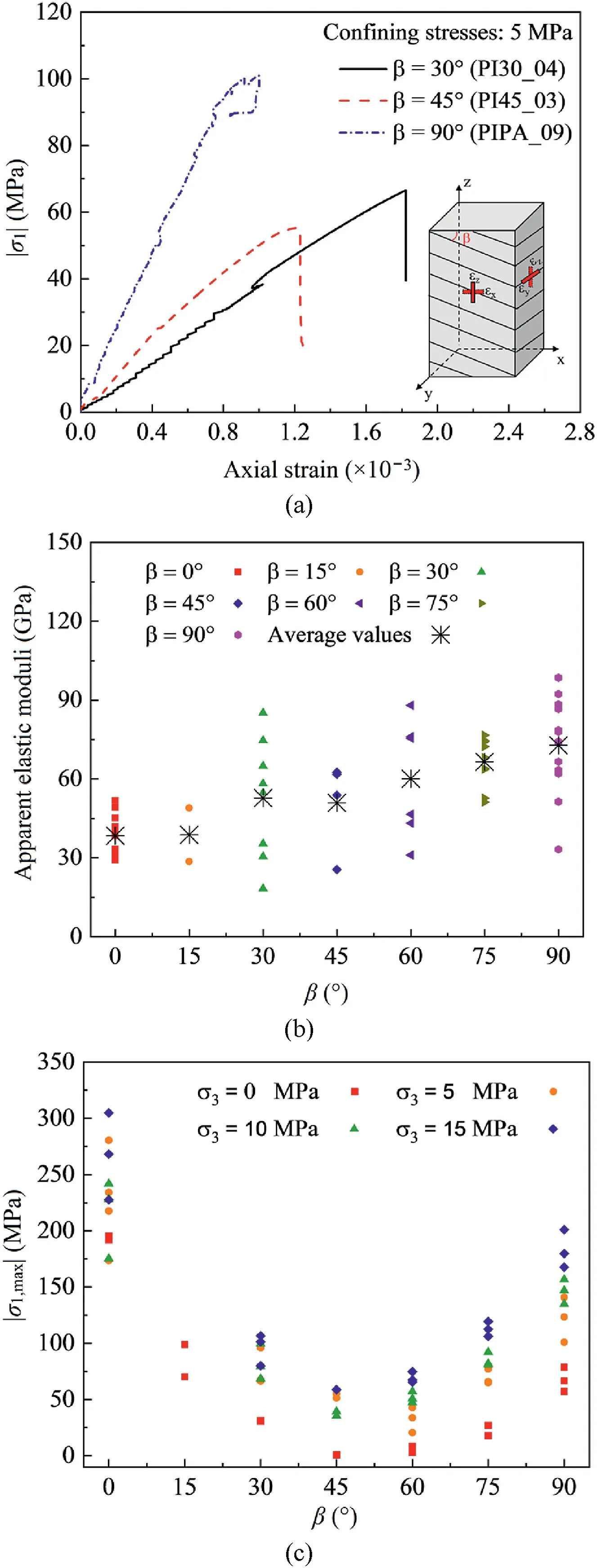
Fig.1.Graphs representing (a) stress-strain curves for slate samples with different anisotropy angles (β=30º,45º and 90º),(b) apparent elastic moduli versus β,and (c)peak compressive strengths(σ1,max)versus β(Modified from Alejano et al.,2021).σ3 is the minor principal stress.

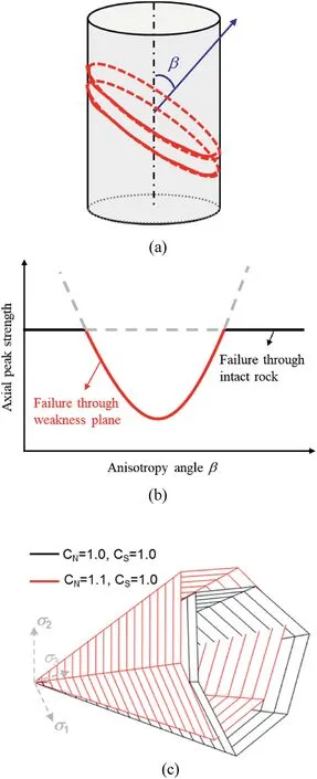
Fig.2.(a) Conceptual representation of a cross-anisotropic geomaterial,(b) Peak compressive strength versus anisotropy angle (β) based on the JPW theory,and (c)Fictitious scaled yield surfaces in the principal stress space in the Mánica’s model,based on the works by Jaeger(1960),Mánica(2018)and Alejano et al.(2021).σ1 is the major principal stress,σ2 is the intermediate principal stress,and CN and CS are the nonuniform scaling factors in the Mánica’s model.

Concerning peak compressive strengths,various failure models have been developed to reproduce the anisotropy of strength.Among all these models,JPW model may be the most commonly used one in interpreting experimental results and numerical modelling.Fig.2a shows the conceptual model of rock samples with planes of weakness.As shown in Fig.2b,two groups of failure criteria are adopted in the JPW model: one associated with the failure through intact rock and the other associated with the failure along the plane of weakness.The minimum strength value obtained from both criteria plays a critical role in the failure mode.The so-called JPW model was initially considered for jointed rocks,but it has been extended for foliated rocks,such as shales and slates(Cho et al.,2012).However,concerning intact rock strength,the predicted strength from the JPW model is forced to be the same when the major principal stress is parallel(β=90º)or perpendicular(β=0º) to the foliation,respectively,which is different from the observed results.Different failure mechanisms result in different strength levels for samples with varied anisotropy angles (β).As observed in laboratory tests of slate from the northwest of Spain(NW Spain slate)and other rocks(see Fig.3)(Donath,1964;Alejano et al.,2021),for the samples cut perpendicular to foliation(β=0º),a double-cone failure can be observed,as in typical isotropic rocks.However,for samples cut parallel to foliation (β=90º),failure through vertical planes combined with local shear bands can be observed.In general,for the rock samples with β=0ºand 90º,the strengths are normally different although the failure mechanism of both cases could be referred to as failure through intact rock(Jaeger,1960).Additionally,for the rock sample with β=45º,the failure mode was typically clean sliding through a foliation plane(Cho et al.,2012;Alejano et al.,2021).

To overcome this limitation of the JPW model,Alejano et al.(2021) proposed the so-called 2 MC-JPW and 2HB-JPW strength models,where two different strength levels can be adapted for samples with β=0ºand β=90º.However,in these improved models,the strength variation along different anisotropy angles is still discontinuous(as in the original JPW model).Moreover,2 MCJPW and 2HB-JPW models have not been implemented yet in any code,and hence,it still needs further research.As a result of all stated above,strength anisotropy is still particularly challenging from the modelling point of view.

On the other hand,some other models have been developed to represent anisotropy of strength.Among all these models,Mánica et al.(2016) and Mánica (2018) proposed a general crossanisotropic plastic model based on a nonuniform scaling of the stress tensor.According to this model,the anisotropic stress space can be obtained by introducing the nonuniform stress scaling factors(CNandCS)to modify the isotropic yield and,thus,account for the cross-anisotropy of strength,as shown in Fig.2c(Mánica,2018).A more detailed explanation of scaling factors (CNandCS) can be found in Section 3.The advantages of Mánica’s approach are that(1)it is able to represent different levels of strength for samples cut perpendicular and parallel to foliation,(2) it is able to represent a continuous variation of the strength along different anisotropy angles.

In addition to the contribution of Mánica et al.(2016) and Mánica (2018),this article (see Section 3) proposes a simple but robust approach to calibrating model parameters and introducing the concept of the dilatancy angle in the constitutive model,which can facilitate its application in rock mechanics.Furthermore,in this study,the smoothed Mohr-Coulomb model is adopted in the numerical implementation,with the aim of improving the numerical reliability and efficiency.Finally,numerical simulations are performed for three types of rocks,i.e.Vaca Muerta shale,Bossier shale and NW Spain slate.Numerical predictions are compared with experimental results,which display a good agreement,validating the proposed constitutive model and approach for calibrating model parameters for the case of the rocks under scrutiny.In addition,the presented model is developed within the framework of the viscoelastic-viscoplastic (VEVP) series constitutive models(Song et al.,2020,2021a,b) in the coupled Thermo-Hydro-Mechanical (THM) CODE_BRIGHT,and therefore,the presented model can be easily extended to simulate coupled THM as well as time-dependent problems.

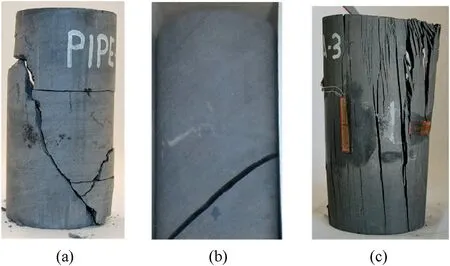
Fig.3.Different failure modes of rock samples (NW Spain slate) with different anisotropy angles: (a) β=0º,(b) β=45º,and (c) β=90º.The confining pressure is 0 MPa.

3.Anisotropic constitutive model for rocks

The viscoelastic-viscoplastic (VEVP) series constitutive models have been proposed by Song(2021)and Song et al.(2020,2021a,b).However,this type of VEVP models can only represent isotropic properties of geomaterials.Hence,this study constitutes a development of the previous VEVP models proposed by Song(2021)and Song et al.(2020,2021a,b),by introducing anisotropic properties in terms of stiffness and strengths.Note that further improvements may be introduced into these models to account for the anisotropy in viscous dashpots and Kelvin models.

3.1.Constitutive model

In order to represent the anisotropic stiffness and strength for geomaterials,an alternative anisotropic constitutive model is presented in this study.As shown in Fig.4,the adopted anisotropic constitutive model consists of an elastic spring and Perzyna’s viscoplastic model.The generalised Hooke’s law is used to describe the reversible elastic constitutive relationship (Lechnickij and Lekhnit skiĭ,1963;Wittke,1990),while Perzyna’s viscoplastic model is used to represent the irreversible strain.Global(x,y,z)and local(1,2,3) coordinate systems are needed to describe the crossanisotropic behaviour of geomaterials,as shown in Fig.5.The global coordinate system(x,y,z)first rotates around thez-axis for the angle of α,and then around they-axis for the angle of β,to obtain the local coordinate system(1,2,3).Therefore,for cases of bedding plane parallel to the 1-o-2 plane as referred in this article,β should be the same as the anisotropy angle of rock samples.

Experience showed that the irreversible strains and the associated stress redistribution might heavily depend on time (Wittke,1990).Thus,the viscoplastic model may be appropriate to represent the behaviour of geomaterials.Moreover,the time-dependent viscoplastic model can be simplified to the time-independent constitutive model by adjusting the viscosity (Fig.4),and therefore,the viscoplastic model is used.Due to the lack of experimental data representing the time-dependent behaviour of the studied specimens,no time-dependency is considered in this research.However,the proposed approach can be easily extended to simulate the time-dependent cross-anisotropic behaviour of geomaterials.

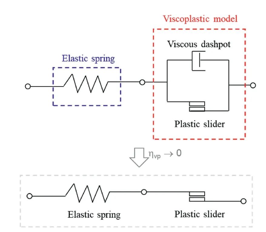
Fig.4.Adopted anisotropic constitutive model for rocks.ηvp is the viscosity in the viscoplastic model.

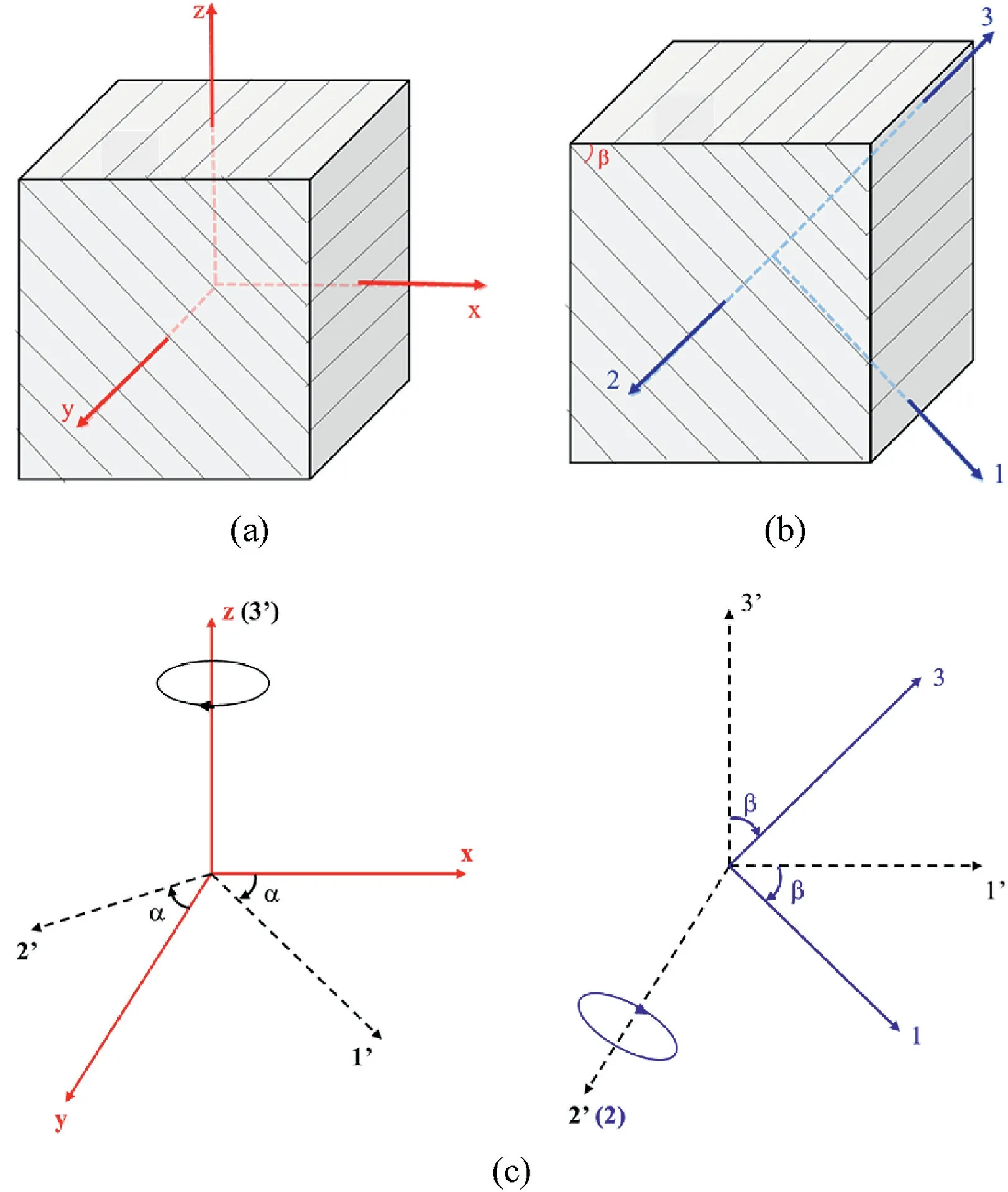
Fig.5.(a)Global coordinate system(x, y, z),(b)Local coordinate system(1,2,3),and(c) Angles in the transformation matrix,based on the work of Wittke (1990),Mánica et al.(2016) and Mánica (2018).α represents the first rotation around z-axis,and β represents the subsequent rotation around the y-axis.

The total strain rate tensor of the proposed anisotropic constitutive model,dε/dt,can be decomposed into components describing the reversible (caused by the elastic spring,εe) and irreversible(caused by the viscoplastic model,εvp)parts,as shown in Eq.(1).Note that a viscoplastic solution which is close to the‘true’ purely plastic solution can be obtained by sufficiently decreasing the viscosity ηvpto be 0 (Alonso et al.,2005).

whereGis the potential,Fis the failure criterion,and φ(F)=Fmwithmrepresenting stress power (Perzyna,1966;Mánica,2018;Song,2021).

The generalised Hooke’s law could describe the elastic constitutive relationship of cross-anisotropic rocks (Payne and Lekhnitskii,1964;Wittke,1990;Alejano et al.,2021),as shown in Eq.(3).For cases where the global coordinate system (x,y,z) coincides with the local one (1,2,3),the local elastic compliance matrixis the same as the global elastic compliance matrixTherefore,Eq.(3)can be simplified to Eq.(4)for this case.

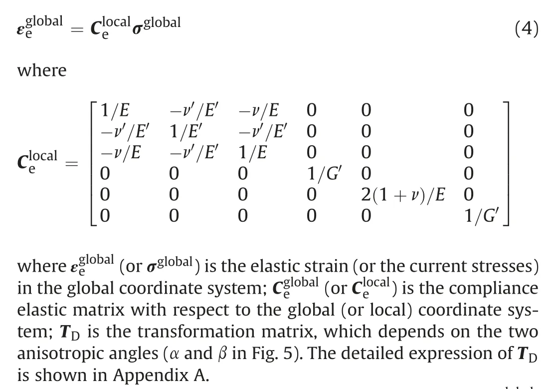
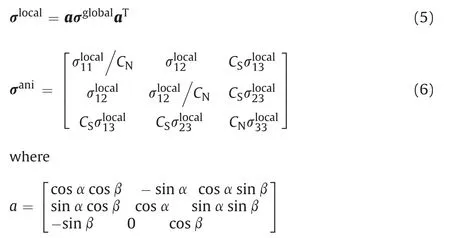
To represent the strength anisotropy,three stress spaces(σglobal,σlocaland σani)need to be introduced(Mánica et al.,2016;Mánica,2018).The stress space in the global coordinate system(σglobal)can be transferred to the local stress space (σlocal),using the transformation matrix ‘a’ (Eq.(5)).Moreover,the anisotropic stress space(σani)can be obtained by introducing the nonuniform stress scaling factors (CNandCS),as shown in Eq.(6).Note that the anisotropic strength can be simplified to the isotropic strength whenCN=CS=1 (Mánica,2018).

A non-associated flow rule is used in this model.The expressions of failure criterion and plastic potential of the adopted Mohr-Coulomb model are shown in Eqs.(7) and (8),respectively.

wherecand φ are the cohesion and friction angle,respectively;ψ is the dilatancy angle;represent the mean effective stress,the second invariant of the deviatoric stress tensor,and the Lode angle in the anisotropic stress space (σani),respectively.

3.2.Calibration of model parameters

In the adopted anisotropic constitutive model,there are five independent elastic constants(E,E′,υ,υ′,G′),and four independent strength parameters (c,φ,CN,CS).Time-dependency is not considered,and thus,a small enough value of ηvpshould be adopted (Song,2021).Based on numerous tests,ηvpis adopted as 100 MPa5s in this research,withm=5.No dilatancy is considered.However,at least in CODE_BRIGHT simulations,null dilatancy(ψ=0º) might result in numerical difficulties.Therefore,a very small value of dilatancy (ψ=0∙01º) has been adopted in these examples.A simple approach for calibration of the model parameters is proposed and described in this section.

As shown in Figs.6 and 7,the stress-strain curves of anisotropic rock samples can be obtained using strain gauges glued in the appropriate directions.The relationships between the five transversely isotropic elastic constants (E,E′,υ,υ′,G′) and Δε/Δσ are displayed in Eqs.(9)-(11).

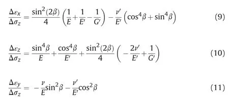
Using the same approach described in former publications(Barla,1972;Worotnicki,1993;Amadei,1996;Chen et al.,1998;Talesnick and Bloch-Friedman,1999;Hakala et al.,2007;Cho et al.,2012;Alsuwaidi et al.,2021),two elastic moduli (E,E′)and two Poisson’s ratios (υ,υ′) can be calculated from rock samples of β=0º(Fig.6a) and β=90º(Fig.6c).After that,the stress-strain curves obtained from samples of 0º<β<90º(Fig.6b) can be used to determine the shear modulus perpendicular to the isotropic plane (G′).Finally,five independent elastic constants (E,E′,υ,υ′,G′) can be determined.A detailed description of the approach used to derived the elastic constants can be found in the literature (Barla,1972;Worotnicki,1993;Amadei,1996;Chen et al.,1998;Talesnick and Bloch-Friedman,1999;Hakala et al.,2007;Cho et al.,2012;Alsuwaidi et al.,2021).

Then,the four independent plastic parameters(c,φ,CN,CS)can be evaluated using the Generalised Reduced Gradient non-linear algorithm (GRG method) (Maia et al.,2017),based on all available test results for each type of rock under study,as shown in Fig.8.As commented in Mánica et al.(2016)and Mánica(2018),CNcontrols the difference between the strengths of cases for β=0ºand β=90º,whileCSaffects the strength for samples of 0º<β<90º.Note again that the anisotropic strength model can be simplified to the isotropic one whenCN=CS=1.

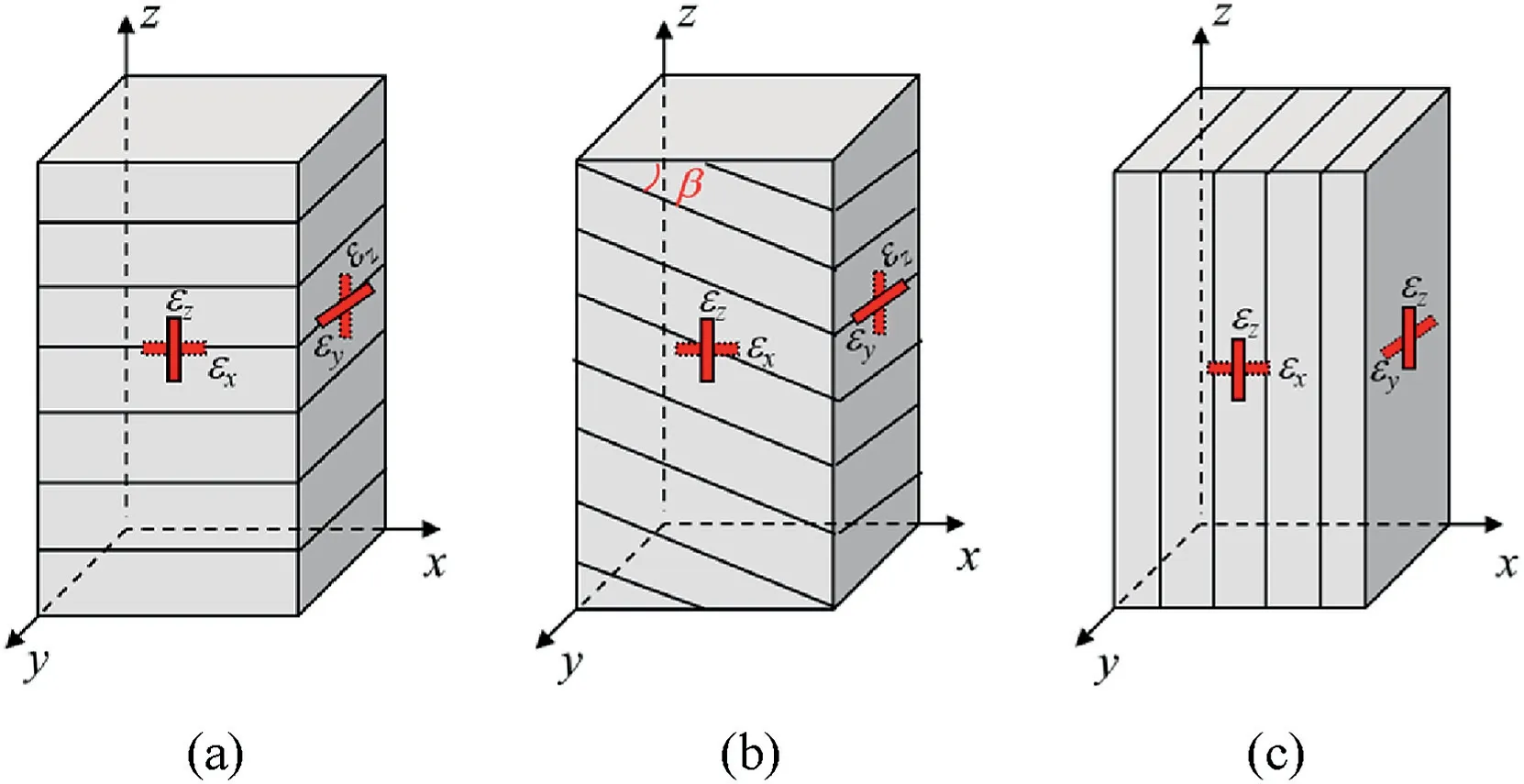
Fig.6.Conceptual model of rock samples with different anisotropy angles: (a)β=0º,(b) 0º <β <90º,and (c) β=90º.

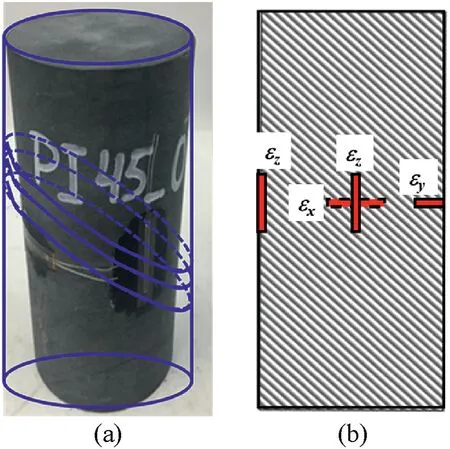
Fig.7.The recommended locations of strain gauges in the laboratory tests.

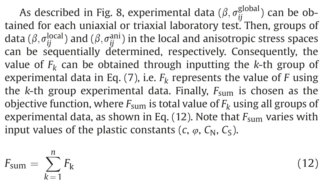
In the determining process,an iteration of the GRG method is carried out,which varies the plastic parametersc,φ,CNandCSto obtain the optional(final)plastic constants,whereFsumis closest to zero.Consequently,the final values of plastic constants(c,φ,CN,CS)can be output.Note that the output values of plastic parameters may depend on the initial values and boundary conditions set for the GRG method.However,the finally obtained values are visually checked to be reliable,physically acceptable numbers,consequent with observations in test results.

3.3.Numerical implementation

The presented anisotropic constitutive model (Fig.4) has been implemented into finite element method software CODE_BRIGHT(Olivella et al.,2021).CODE_BRIGHT is developed at the Universitat Politècnica de Catalunya(UPC)and works in combination with the pre-/post-processor GID.GID has been developed by the International Centre for Numerical Methods in Engineering (CIMNE).

The total strain rate of the presented anisotropic elasticviscoplastic model can be decomposed into elastic (/dt)and viscoplastic (/dt) parts,with respect to the global coordinate system,as shown in Eq.(13).

The strain rate of the elastic spring can be expressed as

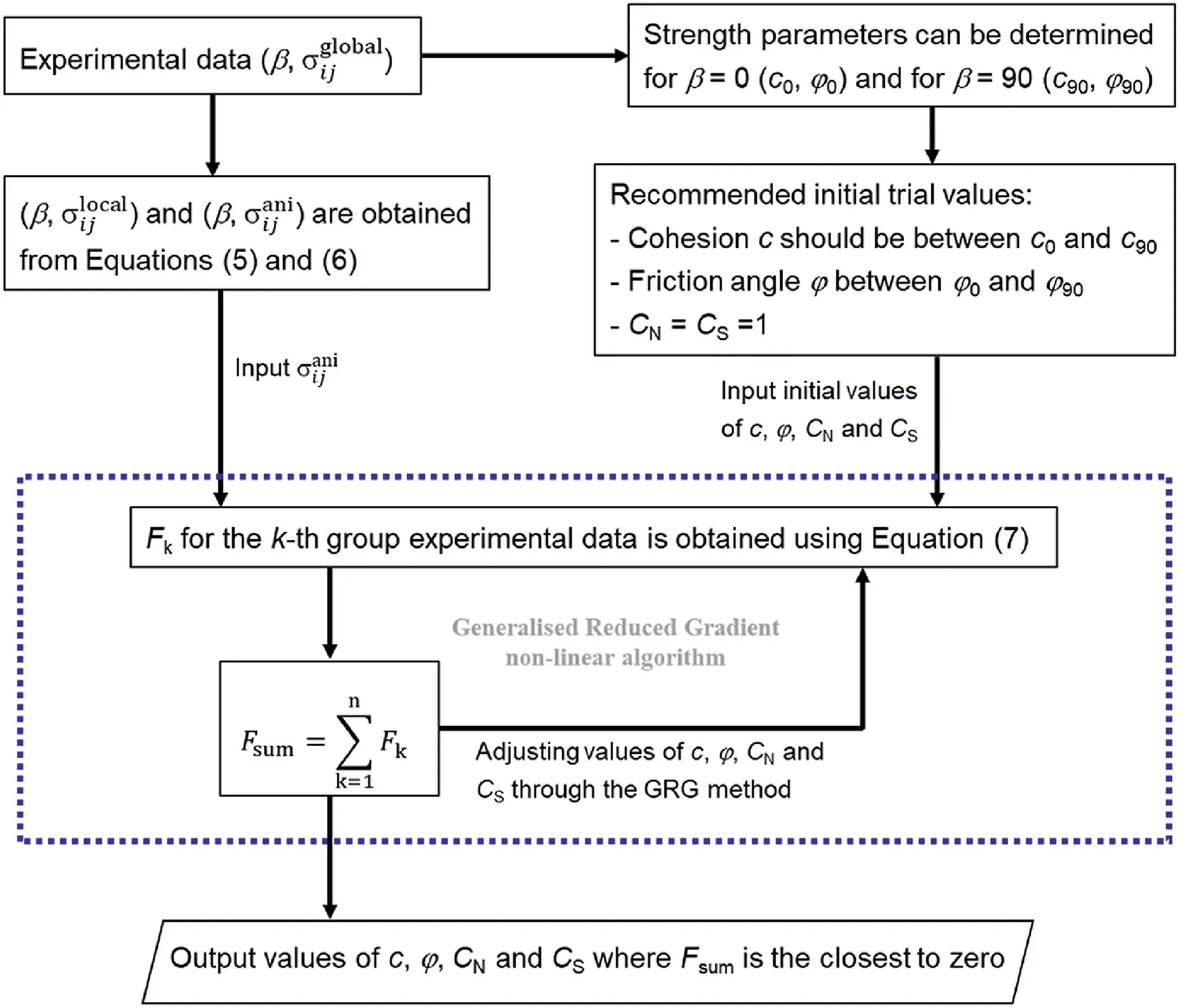
Fig.8.Process of determining the strength parameters.

The derivative of the strain rate of the viscoplastic model with respect to the global stress tensor (σglobal) can be expressed as

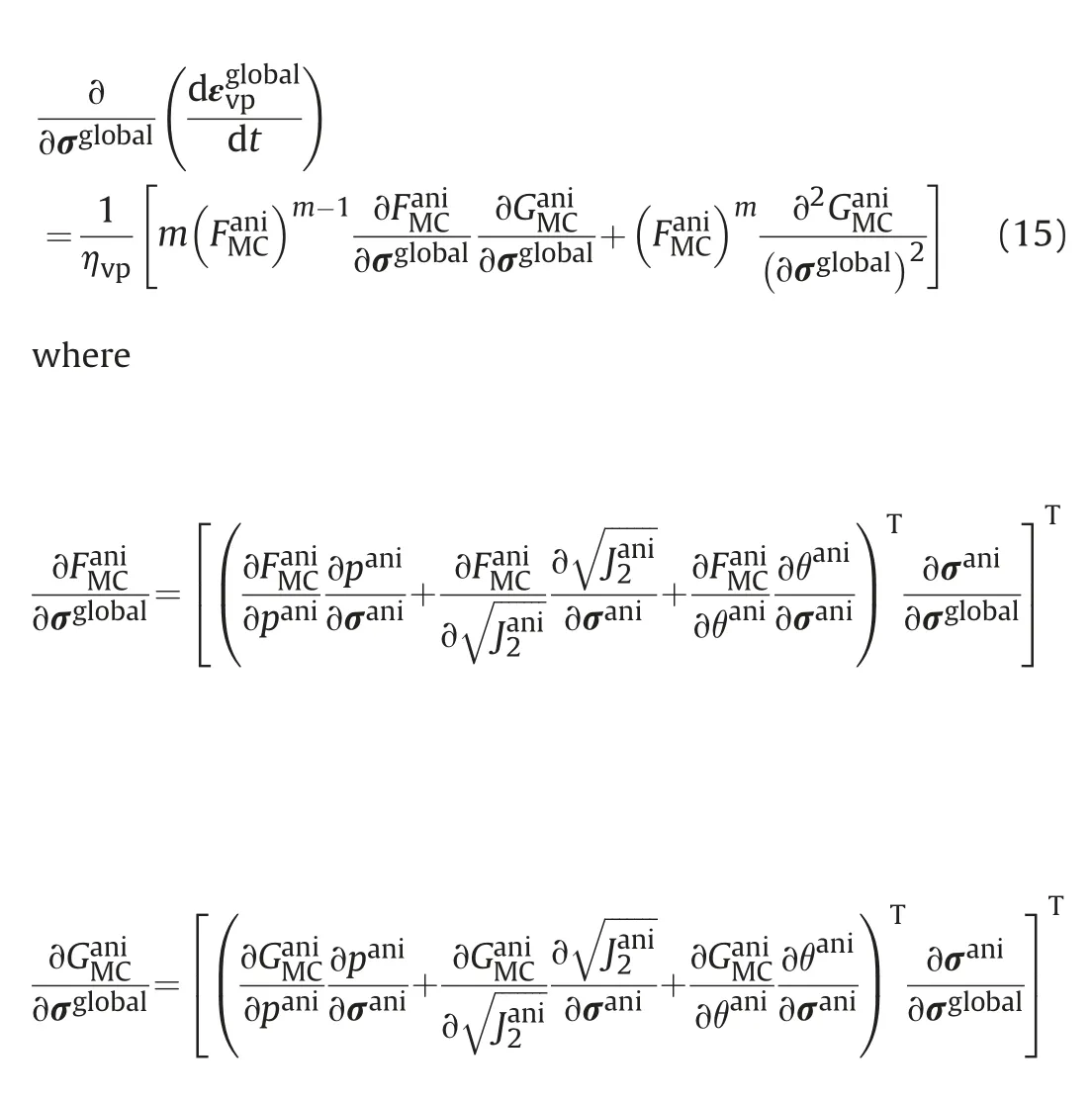
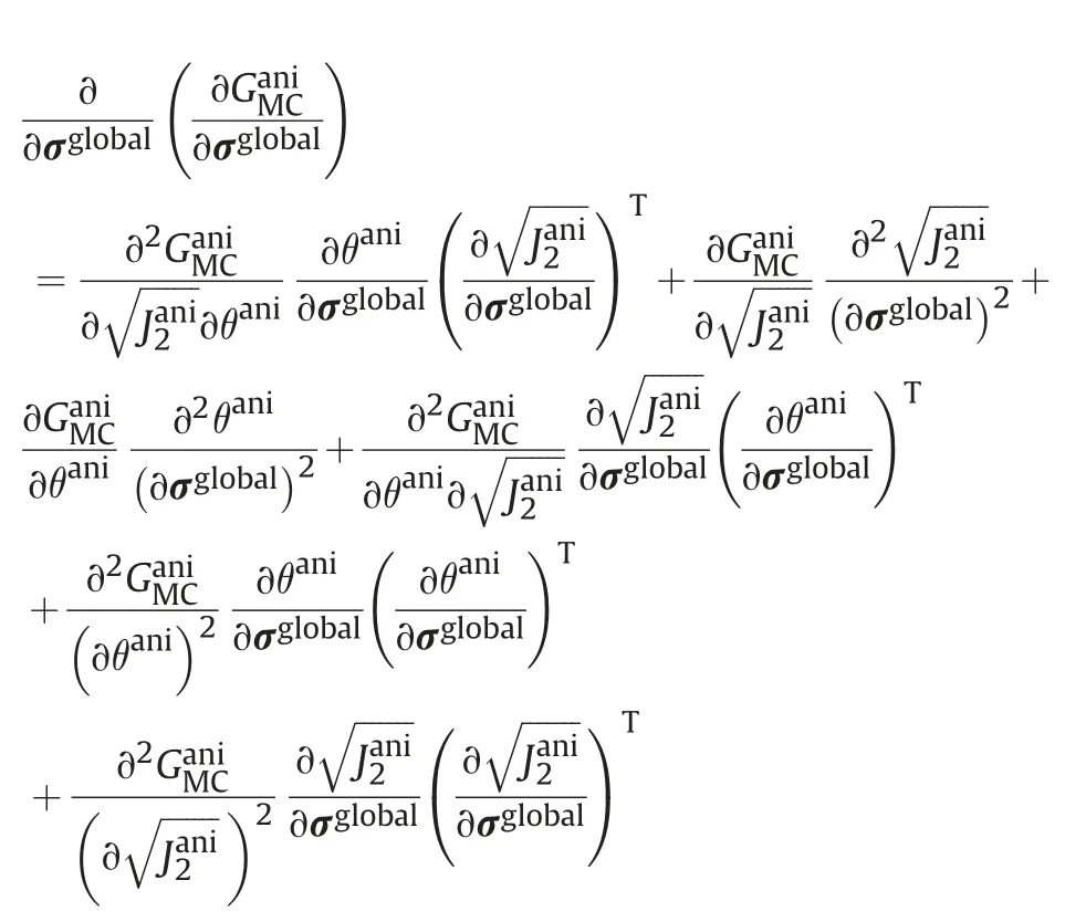
Due to the gradient discontinuities of the yield surface and the plastic potential,numerical calculations may meet numerical inefficiency when using the standard Mohr-Coulomb model in Eqs.(7) and (8) (Song et al.,2020).Therefore,the smoothed Mohr-Coulomb model (Abbo and Sloan,1995;Song et al.,2020) is adopted to improve numerical efficiency and reliability,as shown in Eqs.(16) and (17).

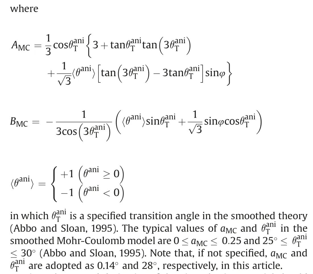
Since the second derivative of the viscoplastic potential should also be continuous,the C2 smoothed theory(Abbo et al.,2011;Song et al.,2020) is used to smooth the potential of the viscoplastic model.The adopted smoothed potential can be expressed in Eq.(18).The alternative form ofKG(θani) in the vicinity of the singularities can be expressed in Eq.(19).

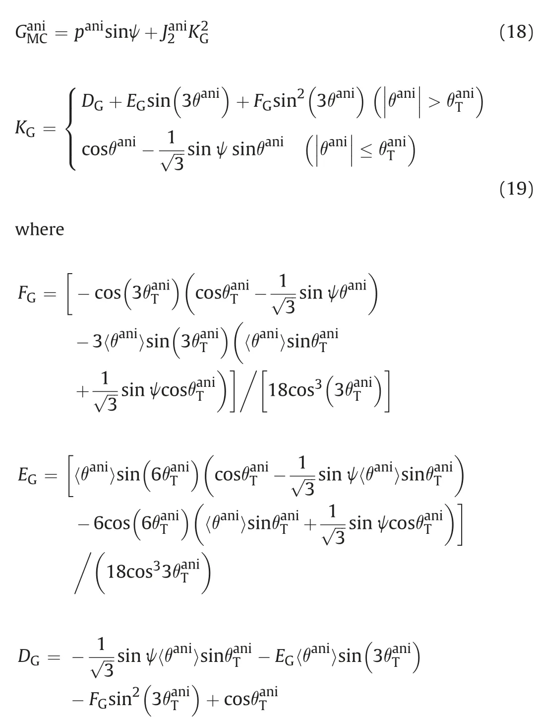
Eqs.(16)-(19) are adapted from the smoothed approximation(C1 and C2 smoothed theories)by Abbo and Sloan(1995)and Abbo et al.(2011).

4.Numerical simulations of anisotropic behaviour of rocks

In this section,numerical simulations of uniaxial and triaxial tests are performed on three types of rocks using the anisotropic constitutive model presented in Section 3.Comparisons between numerical and experimental results are carried out for Vaca Muerta shale(Section 4.1),Bossier shale(Section 4.2)(Ambrose,2014)and NW Spain slate (Section 4.3) (Alejano et al.,2021),in terms of stress-strain curves,apparent elastic modulus (Eθ),apparent Poisson’s ratios (υθand) and peak compressive strengthsIn this section,the sign conventions are defined as negative for tension and positive for compression.For consistency with experimental results and in line with the typical convention adopted in rock mechanics studies,positive is defined as opposite to the direction of the coordinate axis.

Concerning sample preparation,it is challenging for shales and slates.During the process of shale sample preparation,shale cores with significant microcracks were treated with low-viscosity epoxy externally,vacuum suctioned to fill the external microcracks,and cured.Slate samples were prepared with the assistance of a saw disk machine (CEDIMA model CTS-265,400 mm radius disk),a drilling machine(WEKA,model DK22)and a grinding machine.To obtain these slate cores,40 kg slab-like blocks have to be the first cut to produce a base that provides the desired schistosity orientation,and then these properly positioned blocks were cored.It is relevant to mention that cutting of these oriented samples was not an easy task,and it was time-consuming.Thus,in the process of coring,numerous cores were broken,particularly when the foliation formed angles of 15ºand 30ºwith the sample bases since the drilling process generate shear stresses that produce breaking of the samples.More than twice the typical quantity of rock material(with granite or sandstone)was needed to produce the roughly 90 tested samples.Note again that the experimental data of stressstrain curves of NW Spain slate are presented in this article for the first time.

4.1.Vaca Muerta shale

Ambrose (2014) carried out 21 uniaxial and triaxial tests for Vaca Muerta shale.In this section,numerical simulations using CODE_BRIGHT are performed to fit these laboratory results from Ambrose (2014).The numerical model used (Fig.9a) is a threedimensional(3D)cylindrical model with a diameter of 0.055 m and a height of 0.11 m.

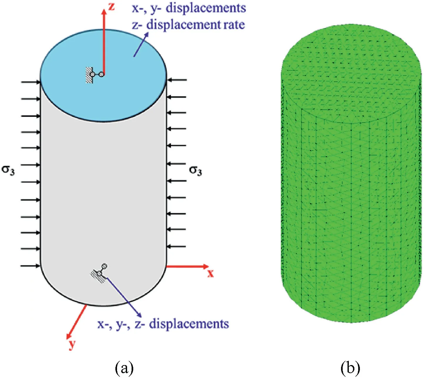
Fig.9.Uniaxial and triaxial numerical tests: (a) Basic features and boundary conditions (conceptual model),and (b) Mesh with 16,980 tetrahedral elements.

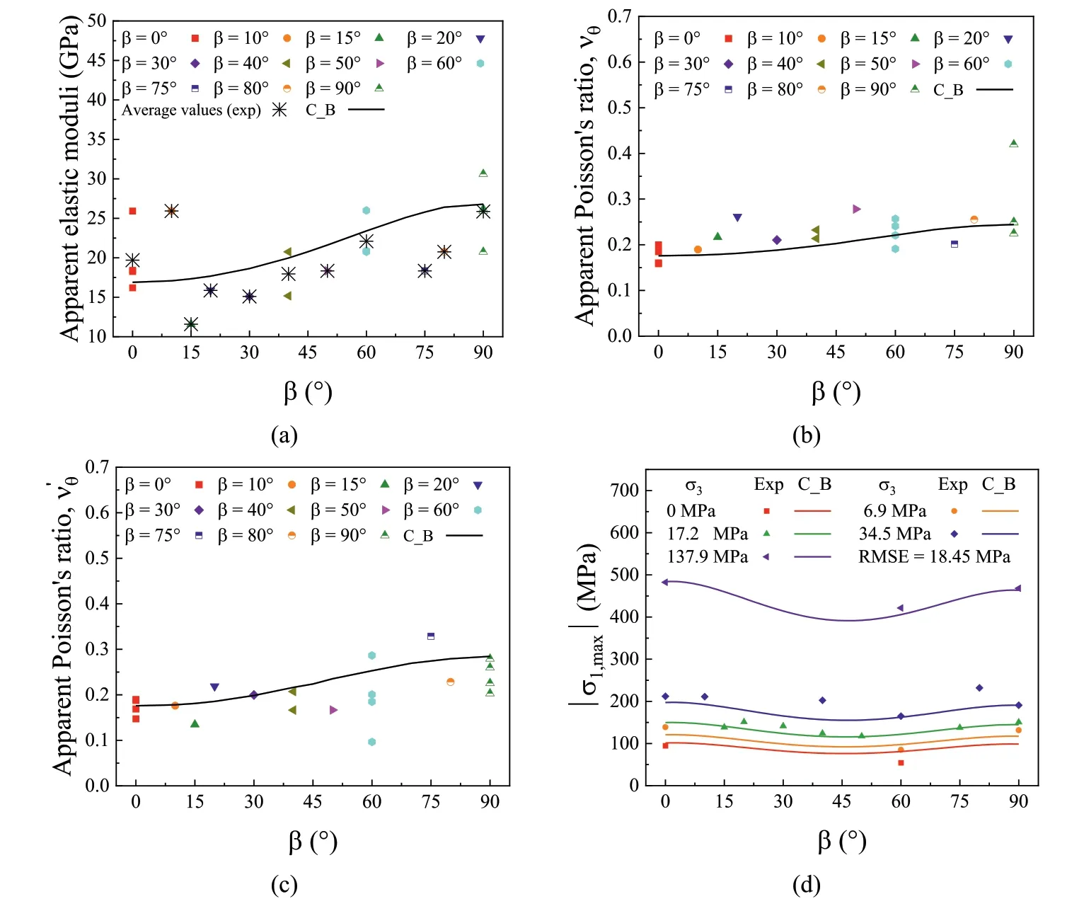
Fig.10.Comparisons of (a) apparent elastic modulus (Eθ),(b) apparent Poisson’s ratio (υθ),(c) apparent Poisson’s ratio (),and (d) peak strength results between numerical and experimental results.‘C_B’ represents the CODE_BRIGHT results.‘Exp’ represents the experimental results.Experimental data are obtained from Ambrose (2014).

Concerning boundary conditions,along the bottom boundary of the model,all displacements are restrained.Along the top boundary,a constantz-displacement rate 1 × 10-7m/s is applied,consistent with that typically applied in laboratory tests,while displacements in thex-andy-directions are restrained.Note that the obtained peak strength is independent on the loading rate in this case since time-dependency has not been considered in the simulations.Finally,on the lateral boundary,a constant radial confining stress (σ3) is applied,representing the actual confinement in the cylindrical sampler walls,applied through fluid pressure on the sample enclosed in a rubber sleeve.

A mesh with 16,980 tetrahedral elements has been considered(Fig.9b),sufficiently accurate and resulting in an acceptable computation time.Table 1 lists the input parameters.

Fig.10a-d shows the comparison of apparent elastic modulus(Eθ),apparent Poisson’s ratio(υθ),apparent Poisson’s ratio(),and peak compressive strengthrespectively,for Vaca Muerta shale between numerical predictions (in terms of lines) and experimental data (in terms of points).Note that apparent elastic modulus (Eθ) is the observed stiffness response of the sample,which can be computed as Δσz/Δεz;the apparent Poisson’s ratios(υθand)can be computed as υθ=-1/(Δεz/Δεy)and=-1/(Δεz/Δεx).A good agreement concerning stiffnesses and strengths between CODE_BRIGHT results and experimental data can be observed.The root mean square error (RMSE) value of numerical predictions to fit experimental results of Vaca Muerta is 18.45 MPa.As a comparison,the RMSE values of the JPW model and the Pariseau’s model to match experimental data of the Vaca Muerta shale are 12.8 MPa and 16.5 MPa,respectively(Ambrose,2014).The smaller the values of the RMSE is,the better the agreement between experimental data and the values of prediction is.Therefore,based on the obtained RMSE values,it can be concluded that the adopted anisotropic strength model can reasonably represent the stress-strain anisotropic behaviour of Vaca Muerta shale.

In addition,Fig.11 presents the comparisons of stress-strain curves of Vaca Muerta shale between numerical and experimental results for six samples.A good agreement of stress-strain curves between numerical predictions obtained from CODE_BRIGHT simulations and experimental data obtained from laboratory tests can be observed,validating that the proposed numerical approach and the adopted transversely isotropic stiffness constitutive model can reasonably represent the anisotropic deformability of Vaca Muerta shale.

4.2.Bossier shale

Ambrose (2014) carried out 36 uniaxial and triaxial tests for Bossier shale.In this section,numerical simulations are performed to fit the laboratory results of Bossier shale from Ambrose (2014).The geometry,conditions and mesh of the numerical model are the same as those described in Section 4.1(Fig.9).The input parameters are listed in Table 1.

Table 1 Input parameters of the adopted anisotropic constitutive model.

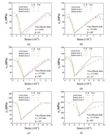
Fig.11.Comparison of stress-strain curves of Vaca Muerta shale between numerical and experimental results for six samples.Experimental data are obtained from Ambrose(2014).Radial strains 1 and 2 represent εy and εx,respectively.

Fig.12 presents the comparison of Bossier shale in terms of stiffness(apparent elastic modulus and apparent Poisson’s ratios)and peak strength between numerical predictions (in terms of lines)and experimental data(in terms of points).A generally good agreement between CODE_BRIGHT results and experimental results can be observed.Moreover,the RMSE value of the adopted anisotropic model of Bossier shale is 28.46 MPa.As a comparison,those of the JPW model and Pariseau’s model are 28.8 MPa and 22.4 MPa,respectively.Therefore,it can be concluded that the numerical predictions can accurately represent the stress-strain response of Bossier shale samples tested in the laboratory.For further validation of the numerical results of stiffness,Fig.13 presents the comparisons of stress-strain curves between CODE_BRIGHT results and experimental data.It can be observed that the numerical prediction can reasonably represent the anisotropic deformability of Bossier shale.

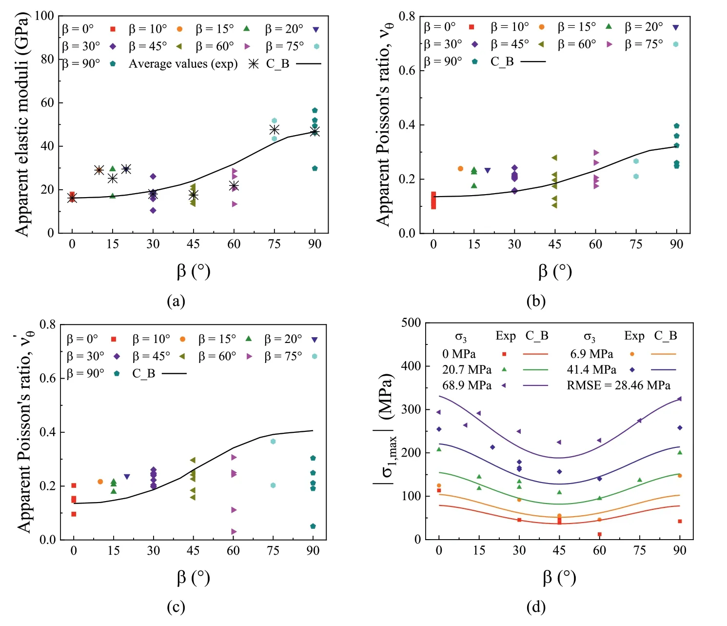
Fig.12.Comparison of(a)apparent elastic modulus(Eθ),(b)apparent Possion’s ratio(υθ),(c)apparent Possion’s ratio(),and(d)anisotropic peak strength results of Bossier shale between numerical and experimental results.Experimental data are obtained from Ambrose (2014).

4.3.NW Spain slate

Numerous laboratory tests were performed on slate samples in a previous study by Alejano et al.(2021).The slate material was acquired from a quarry site in O Barco de Valdeorras,sited in the northwest of Spain.Geologically,the chosen slate belongs to the Luarca series,an Ordovician metamorphic geological level with marked foliation and high consistency.67 compressive uniaxial and triaxial tests were performed on standard rock specimens cut in different directions with foliation and four gauges each to obtain the stress-strain curves.The original data of peak strength and the stress-strain inverse slopes (Δε/Δσ) for all the available samples can be found in Alejano et al.(2021).In this section,a comparison of the peak strength of all available slate samples between numerical predictions and laboratory tests is carried out.Then,the numerical and experimental results are compared to analyse the prediction capabilities of the proposed approach in terms of anisotropic stiffness and strength.

The numerical model geometry and mesh are the same as those described in Section 4.1 (Fig.9).Concerning the boundary conditions,in this case,a constantz-displacement rate of 5×10-8m/s is applied along the top boundary,since slates exhibit stronger stiffness and,hence,smaller applied displacements rates benefit the numerical stability.Table 1 contains the input parameters of the proposed constitutive model.Fig.14a-c shows a good comparision of apparent elastic modulus (Eθ) and apparent Poisson’s ratios (υθand) between numerical prediction using CODE_BRIGHT and experimental data.The JPW model is adopted to explain the anisotropy of the strength of slate,as shown in Fig.14d,with its RMSE value of 37.5 MPa (Alejano et al.,2021).However,the JPW model cannot reproduce the discrepancies of peak strengths for samples of β=0ºand β=90º(Alejano et al.,2021).Moreover,there are discontinuities in the JPW model because two different criteria are adopted for failures along the plane of weakness and the intact rock (as discussed in Section 2).Therefore,to some extent,the JPW cannot accurately represent experimental results of strength.

As an alternative,the adopted anisotropic constitutive model has been used to represent the experimental data of strength for slate.Fig.14e presents the curve-fitting results based on the proposed anisotropic constitutive model (RMSE=37.19 MPa).The RMSE values between the JPW and the adopted anisotropic constitutive models show no significant difference,meaning that both models can predict experimental data with similar accuracy.However,the proposed anisotropic constitutive model can represent different strengths between samples of β=0ºand β=90º.In addition,this constitutive model represents a continuous strength variation with different anisotropy angles,which is different from the ‘discontinuous’ form obtained with the JPW model (Fig.14d).Therefore,it is reasonable to state that the proposed anisotropic constitutive model may represent more realistically the strength anisotropy of rocks than the JPW model.

For further validation,as shown in Fig.15,comparisons of stress-strain curves between numerical predictions obtained from CODE_BRIGHT simulations and experimental data obtained from laboratory tests are carried out,considering various confining stress levels(σ3)and different anisotropy angles(β).For the sake of briefness and clarity,only six stress-strain curves are presented in this section.It can be concluded that the proposed numerical approach can reasonably represent the anisotropic deformability of slate.However,as Fig.15 depicts in comparison with Figs.11 and 13,the numerical results in slate do not fit so well with the laboratory ones,as in the case of shales.The poorer accuracy of these results is attributed first,to the fact that the anistropic approach presented may not perfectly represent the response of the rock,and ultimately,to the natural variability on the response of these rocks.

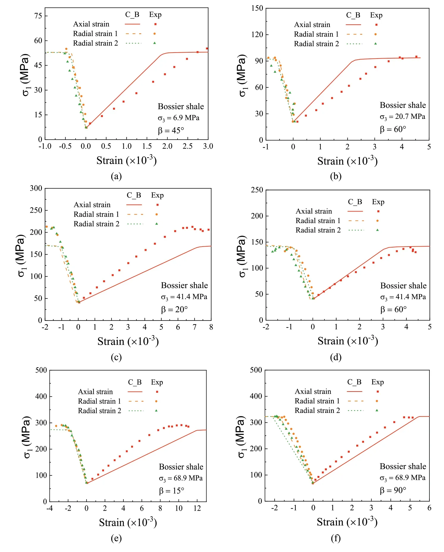
Fig.13.Comparisons of stress-strain curves of Bossier shale between numerical and experimental results.Experimental data are obtained from Ambrose (2014).

5.Conclusions

This article provides an alternative numerical approach for modelling stiffness anisotropy and strength anisotropy for bedded or foliated rocks such as shales or slates.An alternative anisotropic constitutive model is presented and implemented into the finite element method software CODE_BRIGHT to simulate the anisotropic behaviour of geomaterials.Furthermore,a simple approach is proposed to calibrate the model parameters.Finally,comparisons between numerical and experimental results are carried out to validate that the proposed numerical model can represent the actual anisotropic behaviour of rocks.

In the adopted anisotropic constitutive model,stiffness anisotropy and strength anisotropy are incorporated independently.The cross-anisotropic form of Hooke’s law is used to describe the anisotropic deformability of geomaterials.The comparisons of stress-strain curves between experimental and numerical results concluded that the numerical predictions using the crossanisotropic elastic model reasonably match the observed elastic rock sample response.In addition,a nonuniform scaling of the stress tensor is introduced in the plastic model to represent strength anisotropy.In addition,the Mohr-Coulomb model and a non-associated plastic flow rule have been used.

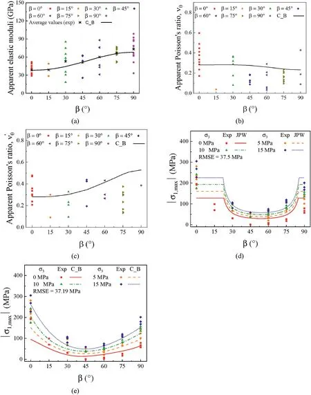
Fig.14.Comparisons of stiffness and strength of slates between experimental data(Alejano et al.,2021)and numerical results using CODE_BRIGHT in terms of(a)apparent elastic modulus (Eθ),(b) apparent Poisson’s ratio (υθ),(c) apparent Poisson’s ratio (),and (e) strengths;and (d) using JPW model in terms of strengths.‘JPW’ represents the prediction using the JPW model,whose input parameters can be found in Alejano et al.(2021).

Numerical simulations of uniaxial and triaxial tests have been performed on Vaca Muerta shale,Bossier shale and NW Spain slate,considering various confining stress levels and different anisotropy angles.A good agreement between the numerical and experimental results is observed,validating that the proposed numerical approach can model the anisotropy of different types of rocks.Moreover,the adopted anisotropic constitutive model can reproduce (i) a continuous strength variation with different anisotropy angles (β),and (ii) different levels of strengths for samples cut perpendicular and parallel to the foliation,which is consistent with the observed experimental results of shales and,particularly,slates,and may model more realistically their behaviours.In conclusion,the presented numerical approach can be used to reasonably represent the stiffness anisotropy and strength anisotropy of foliated and bedded rocks and potentially other geomaterials.

The codes availability

The proposed anisotropic constitutive model has been implemented in the finite element method CODE_BRIGHT (version:Code_Bright_2021_12).The official CODE_BRIGHT versions can be found in the following link: deca.upc.edu/en/projects/code_bright.

Declaration of competing interest

The authors declare that they have no known competing financial interests or personal relationships that could have appeared to influence the work reported in this paper.

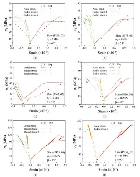
Fig.15.Comparisons of stress-strain curves for slate between numerical and experimental results.

Acknowledgments

The experimental part of the slate in this work was funded by REPSOL S.A.The numerical part of this work was supported by the CODE_BRIGHT Project(International Centre for Numerical Methods in Engineering).The work of the second and fourth authors was possible thanks to the Spanish Ministry of Science and Innovation,who funded the project,awarded under Contract Reference No.RTI 2018-093563-B-I00,partially financed by means of the European regional development fund(ERDF)funds from the European Union(EU).

Appendix A.Supplementary data

Supplementary data to this article can be found online at https://doi.org/10.1016/j.jrmge.2022.04.016.

List of symbols

a Transformation matrix between global and local stress spaces

aMCThe smoothed parameter in the smoothed Mohr-Coulomb model

cCohesion

CN,CSNonuniform stresses scaling factors for modifying the isotropic yield surface

EYoung’s modulus for the directions parallel to the isotropic plane

E′Young’s modulus for the directions perpendicular to the isotropic plane

EθObserved stiffness response of the sample (apparent Young’s modulus)

FYield surface

FkThe value ofFusing thek-th group experimental dataFsumTotal value ofFkusing all experimental data

GPotential function

G′Shear modulus for shear loading in the isotropic plane

mStress power

paniMean stress in the anisotropic stress space

TDTransformation matrix

(x,y,z) Global coordinate system

(1,2,3) Local coordinate system

α Angles in the transformation matrix

β Angles in the transformation matrix;Anisotropy angle for rock samples in the triaxial tests

υ Poisson’s ratio for the lateral strain due to loading parallel to the isotropic plane

υ′Poisson’s ratio for the lateral strain due to loading normal to the isotropic plane

υθ() Apparent Poisson’s ratio

ε Total strain tensor

εxTotal strain in thex-direction

εyTotal strain in the y-direction

εzTotal strain in thez-direction

εeElastic strain tensor

εvpViscoplastic strain tensor

σ Stress tensor

σxStress in thex-direction

σyStress in they-direction

σzStress in thez-direction

σglobalStress tensor in the global coordinate system(x,y,z)

σlocalStress tensor in the local coordinate system (1,2,3)

σaniStress tensor in the anisotropic stress space

σ1The major principal stress

σ2The intermediate principal stress

σ3The minor principal stress

ηvpViscosity of the Perzyna’s viscoplastic model

φ Overstress function

φ Friction angle

ψ Dilatancy angle

θaniLode angle in the anisotropic stress space