Uncertainty analysis of turbulence model in capturing flows involving laminarization and retransition

Hongkang LIU, Shishang ZHANG, Yong ZOU, Wu YUAN,Tanghong LIU, Yatian ZHAO

a Key Laboratory of Traffic Safety on Track of Ministry of Education, School of Traffic & Transportation Engineering, Central South University, Changsha 410075, China

b Joint International Research Laboratory of Key Technology for Rail Traffic Safety, Central South University, Changsha 410075, China

c National & Local Joint Engineering Research Center of Safety Technology for Rail Vehicle, Central South University,Changsha 410075, China

d Computer Network Information Center, Chinese Academy of Sciences, Beijing 100190, China

e School of Aeronautics and Astronautics, Central South University, Changsha 410083, China

KEYWORDS Laminarization;Retransition;Reynolds-averaged Navier-Stokes simulation;Turbulence modeling;Uncertainty analysis

Abstract Flows experiencing laminarization and retransition are universal and crucial in many engineering applications. The objective of this study is to conduct an uncertainty quantification and sensitivity analysis of turbulence model closure coefficients in capturing laminarization and retransition for a rapidly contracting channel flow. Specifically, two commonly used turbulence models are considered:the Spalart-Allmaras(SA)one-equation model and the Menter Shear Stress Transport(SST)two-equation model.Thereby,a series of steady Reynolds Averaged Navier-Stokes(RANS)predictions of aero-engine intake acceleration scenarios are carried out with the purposely designed turbulence model closure coefficients.As a result,both SA and SST models fail to capture the retransition phenomenon though they achieve pretty good performance in laminarization.Using the non-intrusive polynomial chaos method, solution uncertainties in velocity, pressure,and surface friction are quantified and analyzed,which reveals that the SST model possesses much great uncertainty in the non-laminar regime,especially for the logarithmic law prediction.Besides,a sensitivity analysis is performed to identify the critical contributors to the solution uncertainty,and then the correlations between the closure coefficients and the deviations of the outputs of interest are obtained via the linear regression method. The results indicate that the diffusion-related constants are the dominant uncertainty contributors for both SA and SST models. Furthermore, the remarkably strong correlation between the critical closure coefficients and the outputs might be a good guide to recalibrate and even optimize the commonly used turbulence models.

1. Introduction

In many industrial applications, it is a common occurrence that turbulence flow experiences severe acceleration or deceleration caused by rapid changes of the shape or the external environment.For instance,a rapidly contracting pipe or channel always leads to the laminarization of turbulence flow due to the acceleration,accompanied by a strongly Favorable Pressure Gradient (FPG). Once the FPG finishes, the retransition process could subsequently occur with the flow reverting to its turbulent regime.1These phenomena are of much complexity,and a thorough capability in understanding and predicting the behavior and effects of a boundary layer undergoing laminarization and subsequent retransition is of great significance in many engineering applications such as labyrinth seals,rocket engine cooling2and wind or water tunnel.3

Over the past decades, numerous experimental studies and high-fidelity numerical simulations are conducted to investigate the laminarization of turbulence flow subjected to a favorable pressure gradient. Accordingly, some available understanding of its intrinsic mechanism and principles had been achieved, which greatly prompted the full knowledge of the laminarization flow, for instance, Direct Numerical Simulation (DNS) and Large Eddy Simulation (LES) in Piomelli and Prisco et al.4As with the current engineering applications,it is generally acknowledged that RANS models are still the workhorse due to their low computational cost and high robustness in solving the mean flow.5-6As the principal role in today’s CFD landscape,however,many RANS-based models are still suffering great difficulties in capturing the complicated flows above. A widely accepted cognition is that the present RANS-based models possess many empirical formulas and relevant parameters (i.e. closure coefficients) identified by using a combination of heuristic and empirical decision making.7In most cases,the preceding model developers determined some closure coefficients by using dimensional analysis or experimental data of some representative but relatively simple flows, such as homogeneous decaying isotropic turbulence,free shear flow,fully developed channel flow,and so on.8These closure coefficients calibrated by the specified scenarios could not be guaranteed to be universally valid for arbitrary flows and inevitably lead to modeling errors.With respect to the prediction of laminarization flows, Keshmiri et al.9found that using an improper value or formula for Cμhad adverse effects on the performance of the nonlinear k-ε model. Similarly,Menter10pointed out that some subtle changes of the empirical parameters in the SST model could dramatically improve or deteriorate the predictions. Until now, the consensus on their best values or even whether there are definite values is still an open question. For instance, the standard value of Cε2is chosen as 1.92 in k-ε turbulence model in Jones and Launder,11while is tuned artificially to 1.68 and 1.83 in Re-Normalization Group (RNG) k-ε model and k-τ model respectively in Speziale et al.12Considering the inherent uncertainty due to the closure coefficients of the models, naturally, some studies recalibrate them to match with specific flows of interest.According to the work by Gimenez and Bre,13compared with the standard sets, the optimal ones recalibrated could reduce modeling errors between 11%-64% and 8%-45% for RNG k-ε and SA models,respectively.Conclusively,Table 114tabulates the suggested value of the k-ε model closure coefficient collected in previous work8,13,15-20for different flow problems.Obviously, a great discrepancy in values of model coefficients certifies that the uncertainty caused by the diverse values of the closure coefficients ought to deserve more attention for different physical problems.Thus,it can be seen that in-depth comprehension of the impact of the closure coefficients is completely imperative in the RANS-based turbulence modeling.Since RANS-based approaches are still the focus of active research in the foreseeable future,21a more reliable and practical RANS-based simulation framework with a rational evaluation of modeling error is essential to replicate the intricate flow patterns.It is no exception in the prediction of the rapidly contracting channel flow targeted by the current study.

Unfortunately,previous efforts largely neglected to investigate the available engineering methods for predicting themultiple-regime flows involving both laminarization and retransition process. Especially, in terms of the RANS-based models, the effect of their closure coefficients on the solution is still ambiguous.And very limited achievements are acquired in the uncertainty and sensitivity analysis on turbulence models for such rapidly accelerating or decelerating flows.An associated study conducted by Yang and Tucker22analyzed several popular eddy-viscosity models and Reynolds Stress Models(RSM), and their results manifested that the eddy-viscosity models would obtain a much earlier and quicker retransition process after the contraction. In addition, they pointed out that the sensitization to the impact of the large integral length scales would improve the performance of all models. It also demonstrates that the effects of some critical construction ingredients for commonly used turbulence models deserve more in-depth studies.

Table 1 Suggested value of closure coefficients for different flow problems in Shirzadi et al.14

In terms of the specified severely accelerating flows,Uncertainty Quantification (UQ) due to turbulence modeling is currently highly demanded,as well as a further sensitivity analysis to identify the key closure coefficients. In an application circumstance, obtaining a reliable uncertainty estimate could be highly conducive to the decision-making of the design process and method improvement in Bush et al.23In the work of Li et al.24the Bayesian method is employed to recalibrate the closure coefficients of Spalart-Allmaras(SA)turbulence model to improve its performance in the supersonic jet interaction problem, leading to a relative error reduction from 14.99% to 2.95%, through effective Bayesian parameter estimation.Exactly, the urgency and significance for UQ of turbulence modeling are highlighted as one of the two future research directions in the Turbulence Modeling Symposium sponsored by NASA and the University of Michigan in 2017.21And a consensus was reached that the UQ must be better integrated into the CFD processes to determine both the modeling and the numerical errors. In fact, even to this day, one of the widely-accepted perspectives is that the turbulence model is still the dominant source of error in most RANS simulations.25Therefore, in the last few years, more attention has been devoted to the urgent problem. Schaefer et al.26performed UQ for commonly used turbulence models in predicting the axisymmetric transonic bump and the RAE 2822 transonic airfoil flows with the Non-Intrusive Polynomial Chaos (NIPC)theory in Hosder et al.27Gorle´ et al.28also applied this theory to quantify the uncertainties from the Reynolds stress tensor in the RANS simulations of the flow in downtown Oklahoma City. With the same method, Zhao et al.29firstly carried out an uncertainty analysis on the SST model closure coefficients in terms of the aero-heating prediction in hypersonic flows,and then further extended UQ to the RANS-based transition modeling in the hypersonic flows in Zhao et al.30Different from the external flows above, Di Stefano et al.31quantified the uncertainties caused by the model coefficients of common RANS models, including Menter Baseline (BSL) and SST,Spalart-Allmaras and Wilcox k-ω turbulence models, in a scramjet isolator flows. Meanwhile, a sensitivity analysis was conducted to rank and distinguish these critical closure coefficients to the flow solutions.In addition,the Bayesian approach was utilized to explore both model and parameter uncertainty of turbulence models. Oliver and Moser32developed a Bayesian method and applied it to capture uncertainty due to both uncertain parameters and model inadequacy of RANS turbulence models for fully-developed channel flow. Duraisamy et al.33combined Bayesian inversion and Data-Driven techniques to quantify the solution uncertainty due to the construction of turbulence models. Overall, these investigations on the UQ of turbulence model closure coefficients mostly focus on the traditional fully turbulent flows, instead of the multiple-regime flows involving both laminarization and retransition process. Given the insufficient performance, there is still a strong desire for UQ analysis of the current RANS models in terms of the current specified flows.

Therefore, the purpose of our study is to acquire an indepth comprehension of the uncertainty and sensitivity of turbulence model closure coefficients in capturing laminarization and retransition for a rapidly contracting channel flow.Specifically, two widely-used turbulence models are considered: SA one-equation model and SST two-equation model.The potential benefit is to provide a guideline to optimize these closure coefficients for the severe contracting flows involving the process of laminarization and retransition.Thereby, a series of numerical predictions of aero-engine intake acceleration scenarios are conducted with the purposely-designed turbulence model closure coefficients.Using the point-collocation NIPC methods, the flow uncertainties such as stream-wise velocity profile and surface friction are quantified and analyzed in terms of the closure coefficients of the SA and SST model. With the Sobol index,the global sensitivity analysis is performed to identify the critical contributors to the total uncertainty and the correlations between the input parameters and the deviations of the outputs of interest. This study is expected to be conducive to characterizing the modeling uncertainty, and thus improve the performance of current turbulence models in capturing the laminarization and retransition.

2. Numerical methods

The present simulations are carried out by the commercial numerical software ANSYS-FLUENT (Version 18). The incompressible three-dimensional Navier-Stokes equations are solved using the finite volume method. The third-order Monotone Upstream Scheme for Conservation Law(MUSCL) scheme is employed to solve the momentum and turbulence-model terms, and the least square cell-based gradient evaluation is used for computing values of a scalar at the cell faces and secondary diffusion terms and velocity derivatives.34The steady solutions are achieved with the pseudotransient time integration. Two benchmarked models are selected for uncertainty quantification, i.e., the standard S-A model with the strain-vorticity correction and the standard Menter’s SST model. The detailed descriptions of the selected models are given as follows.

2.1. Standard SA one-equation model

The current one-equation turbulent model proposed by Spalart and Allmaras35was designed specifically for aerospace applications that involve wall-bounded flows. With several improvements or corrections in Dacles-Mariani et al.36this model has been extended to the flows with its boundary layers subjected to the adverse pressure gradient.Due to its less computation cost and more numerical robustness in terms of the multi-equation models, the SA model has achieved great success in the predictions of the aerodynamic flow,and is gaining more popularity in turbomachinery applications.

The SA model solves a modeled transport equation for the modified kinematic turbulent viscosity ^ν, whose full formulation is given by.

In these formulas above, the model closure coefficients,including σ, κ, cb1, cb2, cw2, cw3, ct3, ct4and cprod, and their default values are given in Table 2. In addition, a y+-insensitive wall treatment provided by ANSYS-FLUENT34is utilized in the present SA model, covering an intermediate y+value in the buffer layer (y+∈[1,30]).

2.2. Menter’s SST two-equation model

The Menter’s SST turbulence model10combines the standard k-ε model in the outer region and free shear flows, and the original k-ω model of Wilcox in the inner region of boundary layer via the blending function. The improved performance in the prediction of boundary layers subjected to adverse pressure gradient and pressure-induced boundary layer separation makes the SST model one of the most widely and successfully used turbulence models.

The two transport equations for the turbulent kinetic energy k and the specific dissipation rate of turbulence ω in the SST model are described as.

in which, ψ1and ψ2represent the corresponding constants in the original k-ω model and transformed k-ε model respectively.And the functions f1and f2are calculated by,

where f1,f2,Γ1,Γ2and CDKωare internal model functions.The two sets of model closure coefficients, including σk1, σk2, σω1,σω2,β*,β1,β2and a1,and their suggested values are tabulated in Table 3. It is also noted that the y+-insensitive near-wall treatment ω-equation is used, which automatically blends the viscous sublayer formulation and the logarithmic layer formulation based on y+.

3. Uncertainty analysis method

Due to the lack of a comprehensive understanding of turbulence, the closure coefficients for turbulence models could be the sources of result uncertainty in a numerical prediction. In the present study, all the coefficients are treated as epistemicuncertain variables, and the response of the output Quantities of Interests (QoIs) to the input uncertainty is achieved by establishing a surrogate model. Based on the strategy of point-collocation non-intrusive polynomial chaos, the surrogate model can be constructed via the least-squares approach with a number of flow solutions obtained at the sample points.The NIPC establishes the response surface relation between the outputs and input parameters with the computational expense as little as possible,and has been shown great popularity for uncertainty quantification in considerable CFD applications.37,38

Table 2 Standard value of closure coefficients for SA model.

Table 3 Standard value of closure coefficients for SST model.

According to this strategy, a stochastic response value α*(e.g., pressure, surface friction and turbulent kinetic energy)can be decomposed into separable and deterministic components within a series expansion39:

in which αiis the deterministic component, and ψiis the orthogonal basis function corresponding to the ithmode.Here,α*is assumed to be a function of the deterministic vector x and the n-dimensional standard random variable vector ξ. Note that the polynomial expansion of the equation above is supposed to be infinite. However, a normal and practical way is to adopt the truncated and discrete formula, whose number of output modes is determined by

where n is the number of uncertain variables,and p is the order of the polynomial chaos expansion. In the current work, the polynomial order of two (p=2)is selected and has been proven to be reasonable in various CFD applications.40It should be noticed that this truncated formula can be satisfied only when total-order polynomials are used. And thus, the total number of samples Nsis computed by.

where npis the oversampling ratio defined as the ratio of the number of actual samples to the minimum number required.Besides, the sample points (i.e. the optimum collocation points)are obtained by the optimal Latin Hypercube Sampling(LHS).40

With the deterministic CFD evaluations, the response values at the sample points are acquired and subsequently, the surrogate model can be established to approximate the stochastic response surface.By replacing a stochastic response function with the Polynomial Chaos Expansion (PCE) in Eq.(17), the linear system of equations is finally formulated and solved for the spectral models of the random variables.27This system can be computed by.

In this linear system,the multi-dimensional Legendre Polynomials orthogonal in the interval[1.1] are utilized to span the n-dimensional random space for basic functions ψiowing to the bounded distributions of input parameters. Besides, based on the previous validations,40an oversampling ratio np= 2 is considered here to ensure the accuracy of surrogate response surface with a few deterministic samples.

Then,the mean μα*and standard deviation σα*can be evaluated by

As illustrated by West and Hosder,41the Sobol index (global nonlinear sensitivity index)is used to rank the relative contribution of each input parameter to the total uncertainty in the output quantities of interest. Based on the variances in Eq.(23),the Sobol indices are evaluated by Eq.(24).Note that the Sobol indices here are the combined Sobol indices STithat are comprised of both the individual and the mixed contributions from each uncertain variable.

4. Computational details

4.1. Geometry, free-stream and boundary conditions

In the current simulations, the configuration comprised of three sections is a two-dimensional contraction channel studied by Yang and Tucker22with RANS and DNS.Fig.1 shows the schematic of the half channel, including the geometry, the size of these sections, and the details of boundary conditions.The first straight section is placed upstream for fully developed flows, immediately followed by a cosine-shaped contraction section whose contraction ratio Hin/Houtis 0.5.Further downstream, a narrower straight section is utilized. Here, Hinand Houtare the geometrical half channel heights of the upstream and downstream straight section respectively. The details of the geometrical size are tabulated in Table 4. Note that the coordinate origin is on the lower wall upstream to the leading edge of the contraction, δ is the upstream boundary layer thickness (the half-channel height equivalently) of 1 mm, and s represents the length of section L0-L7and Hin. Besides, the streamwise and wall-normal coordinates will be marked with x and y respectively. The no-slip wall boundary condition is imposed at the lower channel wall, while the symmetry and inviscid wall boundary conditions are applied to the upper wall respectively. This treatment is consistent with that by Yang and Tucker.22In the streamwise direction, the pressure inlet boundary condition is used at the entrance of the channel;the downstream exit is given by the standard outflow boundary condition. The flow is simulated with a nominally unit Reynolds number of 3.3 × 106/m, resulting in the maximal upstream centerline velocity Umaxaround 48.26 m/s (i.e. the reference length). Finally, six streamwise stations (S0-S5in Fig. 1) are selected for numerical validation and comparison,covering the upstream (S0), the leading edge (S1), the midplane (S2), and the trailing edge (S3) of the contraction, and the other two (S4and S5) are located further downstream.

4.2. Code validation and grid sensitivity analysis

The benchmark results are examined to verify the numerical methods and boundary conditions used in the current simulations. Moreover, three levels of grid resolution are utilized to preclude grid dependence.Fig.2 schematically shows the computational grid for the channel,and Table 5 lists the details for three grid resolutions. In the streamwise direction, the meshes around the contraction and the second straight section are refined to accurately trace the great variations of flow characteristics in the process of flow laminarization and the subsequent recovery to the turbulent regime. As for the viscous sublayer prediction, the least first grid spacing in the wallnormal is dw= 0.001Hin, corresponding to the minimal y+value of 0.3.According to previous studies,9,22the current grid resolution is sufficient for our RANS modeling. In fact, the y+-insensitive near-wall treatment used here can prominently relax the requirement for the minimal y+. The quantitative comparison of drag coefficient CDand total-pressure coefficients σpfor the grid convergence study is shown in Table 6.The differences between the medium and fine grids are less than 0.5% for both the drag coefficient and the massweighted average total pressure coefficient. Accordingly, the nearly identical results demonstrate that the medium grid is sufficient to accurately capture flow features, and hence will be utilized in the present computations.

Fig. 3 displays the mean streamwise velocity(U)profiles at six streamwise stations for the present RANS predictions,compared with the reference results of RANS and DNS by Yang and Tucker22Here, the mean velocity and wall-normal distance are normalized by the maximal value (Umax) at the inlet profile and the local half-channel height (Hlocal) respectively.As shown in Fig.3(a),the present predictions at the station S0for both the SA and SST model are well compared with the referenced results. Approaching the contraction, the disparities near the edge of the boundary layer gradually enlarge between the RANS and DNS.Downstream of the contraction(S4), however, the RANS methods produce remarkably large discrepancies within the boundary layer. This discrepancy should be ascribed to the intrinsic mechanism of the RANS models, which neglects the lagging mechanism caused by the rapid acceleration.22It is also noticeable that consistently excellent agreements are obtained in our results for all the selected stations with the reference RANS results. Furthermore, Fig. 4 display the streamwise distributions of the peak mean streamwise acceleration parameter Kx,peakand friction velocity uτ. Note that the subscript in indicates the value at the inlet. All the tested turbulence models predict the maximum streamwise accelerations similar to that of the DNS.Downstream of the contraction,the friction velocity decreases successively due to the laminar regime. However, after x/δin= 15, two curves computed by RANS remain essentially horizontal,as shown in Fig.4,and thus result in the enlarging discrepancies between the RANS and DNS.Overall,these predictions with acceptable accuracy are well-matched with the characteristics of the RANS models, which also manifests the credibility of the present simulations.coefficients, which also commonly used in previous related studies in Schaefer et al.26,Di Stefano et al.31and Zhao et al.29For a thorough uncertainty analysis, the results’ sensitivity to the choice of CoV demands more comprehensive investigations, but is outside the scope of the current work.

Table 4 Geometric details.

Table 5 Details for grid convergence.

4.3. Uncertainty quantification details

According to previous studies,the small changes(5%-10%)in the closure coefficients could result in a remarkable improvement or deterioration of the model predictions.10Owing to the heuristic assumption and the imprecision in the modeling,unfortunately, the epistemic intervals for the RANS closure coefficients are still non-conclusive. Consequently, these epistemic intervals in the present study are chosen in accordance with the previous associated work of Schaefer et al.26Tables 7 and 8 tabulate all the closure coefficients of the SA and SST model for all the simulations, respectively, assigning the standard value and their epistemic intervals. Most of the following constraints for the SA model were recommended by Spalart and Allmaras,35while the epistemic intervals for the SST model were employed from Wilcox 2006 k-ω twoequation model. It should also be noted that, in Table 8, the values of some closure coefficients in the SST are different from those in Schaefer et al.26because of the reciprocal relationship.

Finally, emphasis is placed on that the sensitivity results closely depend on the variation ranges of the selected input parameters.In the present study,different Coefficients of Variations (CoV) for the modeling parameters are utilized to approximate the common understanding of the RANS closure

Table 6 Convergence results for three grid sizes.

5. Results and discussion

In this section,the results of the baseline are described to illustrate the essential characteristics of the acceleration flow and its predictions with the RANS methods. Then, the uncertainties due to the closure coefficients are quantified for the SA and SST models respectively. Immediately afterward, the sensitivity analyses are conducted to reveal the critical parameters.Finally,the linear regression method42is utilized to investigate the linear relationships between the closure coefficients and the outputs quantities of interests.

5.1. Baseline results

Fig. 5 shows the spatial distributions of the mean streamwise velocity,acceleration parameter and Turbulent Kinetic Energy(TKE).Here,the mean streamwise acceleration parameter22is defined as

In which v0and Uedgerepresents the kinetic viscosity and the velocity at the edge of the boundary layer. As can be seen from the figure, the mean flow experiences a substantial rapid acceleration through the contraction,and a slight deceleration downstream.The values of Kxgreater than 10-6indicate that,as concluded by Jones and Launder,43no logarithmic region would be observed. Meanwhile, the boundary layer becomes thin firstly and thickens again when it comes to the straight section.Besides,the RANS prediction also shows that the turbulent kinetic energy recovers immediately downstream of the contraction.

The mean streamwise velocity U+profiles in terms of normalized wall normal distance y+at six stations (S0-S5) are plotted in Fig. 6. Both the SST and SA predictions are provided to compare with the DNS22and the Logarithmic law.At the first two stations,all the numerical methods obtain similar turbulent velocity profiles.Once the flow experiences acceleration, nearly the whole profiles exhibit departure from the universal law of the wall, especially for the logarithmic layer.At S3, as shown in Fig. 6(d), a longer linear region appears until its profile extending to the beginning of the logarithmic law.The predictions of the two RANS models imply that they are capable of predicting the accelerating flow. After the contraction, the velocities in the logarithmic-law section recover profoundly but shows great discrepancies with the turbulent state. Observing the flows downstream, these profiles for y+＞10 predicted by DNS continue to rise and progressively deviate from the logarithmic law, clearly indicating the nonturbulent flow.On the contrary,the predictions by two RANS models are much closer to the logarithmic law while owning approximately laminar slopes.

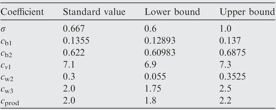
Table 7 Summary of closure coefficients for SA model.

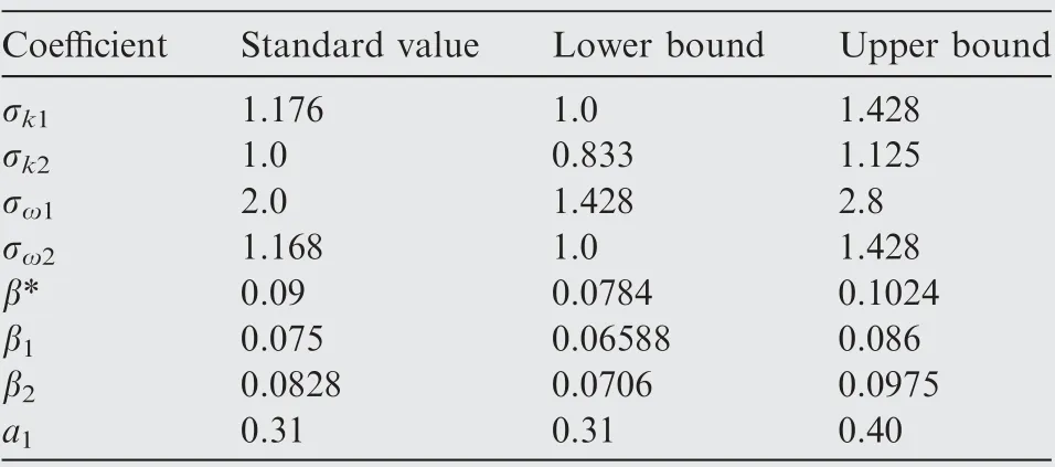
Table 8 Summary of closure coefficients for SST model.

5.2. Uncertainty quantification and sensitivity analysis

The results of uncertainty quantifications and sensitivity analyses for two RANS models are presented in this section.Firstly, some integrated and mass-weighted output quantities such as turbulent viscosity coefficient μt, CDand σpare concerned. Then, the uncertainties of velocity, skin friction and pressure coefficient for the SA and SST models are discussed respectively, followed by the sensitivity analyses in which Sobol indices are introduced to rank the relative contribution of each closure coefficient to the overall uncertainty. Generally, coefficients with higher Sobol indices contribute more to the uncertainty than those with lower Sobol indices.

Table 9 tabulates the results of uncertainty quantification for three output quantities at station S5, containing the baseline, mean value, and its variation interval width. Here, CDis the drag coefficient of the viscous wall.μtand σpare the face mass-weighted turbulent viscosity ratio and total-pressure recovery coefficient respectively, which are computed by

in which φ is the total mass flow rate and ρ is the density. U and A represents the vector of velocity and unit area. φ and φ* symbols the variable and its face mass-weighted value respectively. For both the SA and SST models, the mean values are quite close to their baseline ones, verifying the present UQ computations. Compared with the SA model, the SST model possesses much larger variation interval widths for all the selected quantities. Note that the remarkable disparity of μtfor the two models should be attributed to their intrinsically different mechanisms. Overall, in terms of the incompressible rapid acceleration flows,the SST model is much more sensitive to the variations of their closure coefficients.This conclusion is consistent with the previous results of Schaefer et al.26in transonic wall-bounded flows and Zhao et al.38in hypersonic flows.

To further reveal the critical coefficients, sensitivity analyses are undertaken for turbulent viscosity ratio μt, drag coefficient CDand total-pressure coefficient σp. As shown in Tables 10-12, the corresponding Sobol indices are calculated and listed in descending order. Three closure coefficients of the SA model,i.e.σ,cw2and cv1,could be found to contribute significantly to the uncertainties,and σ makes the greatest effects.In terms of the SST model, σω1can be regarded as the only dominant contributor for CDand σp, different from the four leading parameters for μt.

5.2.1. SA turbulence model

In the following discussion, the output quantities of interest,i.e. pressure coefficient Cpand surface friction coefficient Cf,will be expressed as their mean values with a variation interval width at a 95% Confidence Interval (CI). The epistemic intervals are computed with the standard deviations after the NIPC process.Besides,the maximum and minimum values computed by Monte Carlo simulations are also provided for comparison.

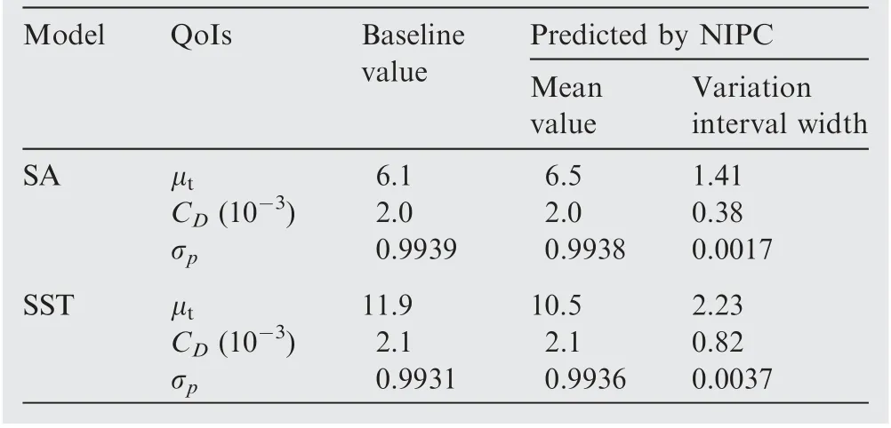
Table 9 Results of uncertainty for specified output quantities.

Figs.7(a)and(b)display the streamwise distributions of Cpand the Sobol indices versus x along the wall, respectively.Through the section of contraction, the differences of Cpvariations for all the training cases are nearly negligible.Then,the variation interval enlarges downstream very slowly.Uncertainties due to closure coefficients make little influence on the pressure for the current flow, especially during the contraction.From the Sobol index distributions in Fig. 7(b), as expected,σ plays a primary role in the contribution of the uncertainty of Cp,followed by cw2.During the contraction,the Sobol index increases for σ but declines for cw2, and then cprodexhibits growing importance during the recovery. With regard to Cf,its distributions and Sobol indices along the wall are shown in Fig.8(a)and(b),respectively.Different from Cp,the uncertainties of Cfexhibit great sensitivity to the closure coefficients,especially in the turbulence recovery flow.Meanwhile,the variation intervals in the contraction section are much smaller dueto the laminarization effect. From Fig. 8(b), the variations of the Sobol index for Cfalso show that σ, cw2and cv1are the top three contributors, and the effects of cw2remarkably decline through the contraction.

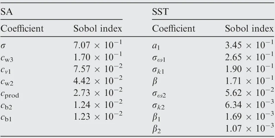
Table 10 Sobol indices for turbulent viscosity ratio.

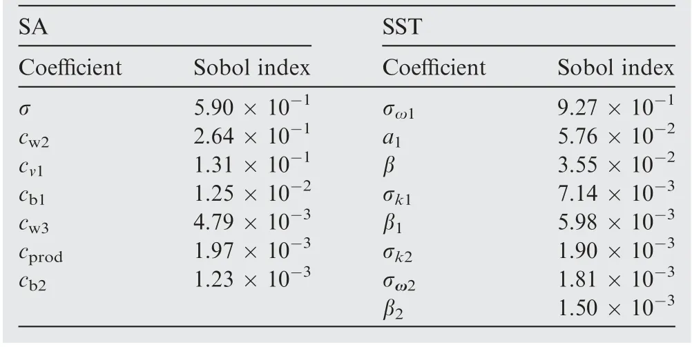
Table 11 Sobol indices for drag coefficient.

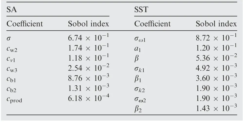
Table 12 Sobol indices for total-pressure coefficient.

To reveal the effects on the boundary layer in the vertical direction, the streamwise velocity profiles for all the training cases at three locations (i.e. S0, S2and S4) are provided in Fig. 9, including the baseline, theoretical solution and DNS data.Observing these profiles at the three stations,we can note that large intervals almost appear in the upper section of the boundary layer, except around the laminarization region.Therefore, it is rational to conclude that while nearly inactive in the viscous sub-layer and rapid acceleration flow for RANS methods, the closure coefficients have great influences on the logarithmic layer. This feature might be ascribed to that the y+-insensitive wall treatment is adopted for the SA model and thus, allows the direct solution of viscous sublayer independent of the uncertainties of model closure parameters.Fig. 10 shows the distributions of Sobol indices versus y+for the streamwise velocity at S0and S4respectively. Apart from these regions below y+= 10, clearly, σ makes great effects in the log-law region,followed by cw2and cv1.However,distinct troughs for σ and cw2, accompanied by an overshoot for cv1, appear among y+∈[70,80] at S0, while at S4, these troughs occur among y+∈[20,30] and cw3produces the overshoot instead of cv1. Obviously, the coefficients σ, cw2and cv1, which are associated with the diffusion term, eddy viscosity destruction and log law intercept calibration respectively,were found to be the significant contributors in the log-law region of the boundary layer. Roughly, it is conjectured that at S0, the rise of Sobol index of the cv1could partially contributes to the decrement of σ, because its great importance in the eddy viscosity log law intercept. As for S4, because of the unconventional boundary layer caused by the laminarization,cw3which speeds up the decay rate of the destruction term mainly activates near the outer region of the boundary layer.

5.2.2. SST turbulence model

The curves for Cpand Cfin terms of x are plotted in Fig. 11 and Fig. 12, respectively, and the corresponding Sobol indices are provided.The nearly consistent plots can be observed in Cpfor all the training cases,similar to the results predicted by SA in Fig. 7. However, the predictions for Cfexhibit many great uncertainties due to the variations of model coefficients, especially around the area of turbulence recovery flow immediately behind the contraction. Apparently, the SST model possesses more sensitive to the closure coefficients compared with the SA. Meanwhile, the results shown in the two figures indicate that the ω diffusion constant σω1is almost the dominating contributor for the uncertainties during the entire channel flow.Only downstream of the contraction,i.e.x/δin=14,the Sobol indices for the stress-limiter coefficient a1firstly enlarges and then declines slightly, though at a relatively low level (around 0.2).In addition,uncertainty contributions due to the remaining closure coefficients can be nearly neglected. Taken together,these results suggest that the turbulence recovery process predicted by the SST model should substantially emphasize the impacts of the corresponding diffusion constants(σω1and a1).This result is consistent with the finding of previous work on an isolator flow by Di Stefano et al.31

Fig. 13 presents the streamwise velocity profiles at three locations(i.e.S0,S2and S4),providing the baseline,theoretical solution and DNS data for reference.The deviations in the viscous sublayer could be neglected mostly due to the y+-insensitive near-wall treatment as well. Compared with the results above obtained by SA, as expected, remarkably larger intervals can be observed in the logarithmic layer section of the boundary layer. And the training cases tend to underestimate the velocity in the log-law region for a non-laminar flow regime. Besides, the baseline curve at S4(marked by a red dashed line) indicates that the standard values can achieve a prediction closer to the DNS data in terms of these training cases. To clarify the major parameters, Fig. 14 presents the profiles of Sobol indices for all closure coefficients at S0and S4. Overall, the ω diffusion constant σω1plays a dominating role at S0, though a sharp declination happens in the region with y+∈[40,60] where β1suddenly arises. By contrast, many complex variations emerge in the logarithmical layer at S4.σω1extremely decreases at y+∈[20,30] while a1enlarges and immediately plunges. Then a similar phenomenon occurs around y+= 100, in which both σω1and a1substantially decline whereas β1ascends. To deepen understanding, here we only attempt to seek a possible explanation. On one hand,usually the k-ω model is chosen in the region near the wall,exerting their effects on boundary layer structure features.On the other hand,σω1is significantly associated with production term and diffusion term in the ω equation, a larger σω1leads to a greater specific dissipation rate ω near the wall.Besides, as one of the blended parameters used in the calculation of β for the ω equation, β1affects the blended ratio that approximates the time decay of homogeneous isotropic turbulence,26which theoretically happens in the log-law layer. As for a1used in the definition function shown in Eq. (14), it is closely associated with the turbulent eddy viscosity. As a consequence, combining with the distribution of turbulent eddy viscosity at S4in Fig.5,it is conjectured that the uncertainty of a1could influence greater on the velocity profile around y+∈[20,30].

5.3. Linear regression

In this section, the linear regression method42is utilized to illustrate the linear relationships between the closure coefficients and the selected output quantities of interest at station S5. With the sensitivity analysis above, correlation coefficients are calculated to advance the sensitivity analysis. The correlation coefficients approximating 1 or -1 signify the stronger positive or negative correlations respectively.

According to the Sobol indices in Tables 10-12,the critical closure coefficients are selected to demonstrate the correlations. Fig. 15 displays the scatter plots of the top uncertainty contributors(i.e.σ in the SA model)and the output quantities of interest for all the UQ training cases, and the baseline results are provided for comparison. All three selected output quantities show strong linear correlations with σ. Specifically,the μtand CDachieve positive correlation coefficients of 0.839 and 0.783 respectively, while σppossesses a negative value of-0.835.Considering the effects of laminar and turbulent flow on the skin friction,it is rational to conjecture that a larger σ tends to obtain a more turbulent result for the SA model.The currently suggested value can be taken as the relatively conservative one. Similarly,the correlations for the SST model are presented in Fig. 16 with the scatter plots. As a result, the stress-limiter coefficient a1is the major contributor for μt, and the relatively scattered plots indicate a moderate positive linear correlation between them. On the contrary,the CDand σpclearly vary with σω1in quadratic polynomial modes, and the density distributions of these plots signify strong correlations between the outputs and σω1. As σ increases, CDdescends while σpenlarges. Consequently, these specific and strong correlations indicate that the ω diffusion constant σω1can be a good alternative closure coefficient for the improvement of the SST model.To understand this behavior, we seek a possible explanation for the distinct variations.According to the model theory, SST turbulent model utilizes blending function f1to combine the k-ω and k-ε models, as shown in Eq. (15). When f1is equal to one, usually the k-ω model is chosen in the region near the wall, which is closely related to the wall shear stress; otherwise, the k-ε model activates. Because σω1is significantly associated with the production term and diffusion term in the ω equation, a larger σω1leads to a greater specific dissipation rate near the wall.Therefore, the wall shear stress weakens, resulting in the decrement of drag CD. In addition, the loss of total pressure is positively related to the viscous effect near the wall. As a consequence,the σppossesses an opposite variation with CD.

For a thorough investigation, the correlation coefficients for all the closure coefficients and the selected output quantities of interest are presented via the bar graph in Fig. 17(a)and Fig.17(b)respectively. For the SA model, σ and cv1show noteworthy but opposite correlations with the three QoIs.And μtand CDshow similar variations with the closure coefficients.From Fig. 17(b), however, a great difference can be observed in the correlation coefficients for the SST model.CDand σpare mainly dominated by σω1via negative and positive correlations respectively, while μtgreatly depends on five closure coefficients. Considering the importance of closure coefficient calibration, these quantitative correlations can be a good guide to the optimization of the commonly used turbulence models,aiming at attenuating the modeling inaccuracy.

For the current flow,two aspects can be taken into consideration to approach it. Firstly, the Sobol index determines the dominant parameter, and the linear regression results indicate a better value range.For example,according to Fig.16,in the severe acceleration and initial retransition stage, the a1should be maintained at a smaller level, while the σω1increases to a certain extent,to partially lessen the viscous and turbulent diffusion. This treatment that partially adjusts specific model parameters can refer to the work of Yang and Tucker.22But it is also noted that the value determination should depend on the global performance, not only local results. Therefore,more global high-fidelity results are imperative for the current flow. Another approach is to introduce the Bayesian method to recalibrate the closure coefficients.Based on the total Sobol index obtained by the NIPC method, the high-fidelity data such as CDand σpcan be served as calibration values to get the posterior uncertainty of model parameters and QoIs.Meanwhile, the calibration effects of likelihood functions should be systematically evaluated. Similar work can refer to that of Li et al.24In their work, the relative error of the wall pressure predicted by the SA model can be reduced from 14.99% to 2.95% by effective Bayesian parameter estimation for supersonic jet interaction flows.

6. Conclusions

This study conducts an in-depth investigation on the uncertainty and sensitivity of turbulence model closure coefficients in capturing laminarization and retransition for a rapidly contracting channel flow.Two commonly used linear eddy viscosity models including the standard SA and SST models are considered. The potential benefit is to provide a guideline to optimize these model closure coefficients for the flows involving laminarization and retransition. Therefore, a series of numerical predictions of aero-engine intake acceleration scenarios are implemented with the purposely-designed turbulence model closure coefficients. Using the NIPC method,the solution uncertainties are quantified and analyzed in terms of the closure coefficients of the SA and SST model. Finally,the sensitivity analysis is performed to identify the critical contributors to the total uncertainty. With the linear regression method, the correlation coefficients are obtained to indicate the relevance between model parameters and the corresponding performance. The main conclusions are as follows:

(1) The results show that the SA and SST models used here achieve pretty good performance in capturing the laminarization phenomenon while failing to depict the retransition process after the severe flow acceleration.Uncertainty analysis reveals that the SST model possesses many great uncertainties in both fully turbulent and transtional flows. Especially, the logarithmic layers acquire larger uncertainty intervals in terms of the velocity profile.

(2) The Sobol indices indicate that the diffusion-related constants are the dominant uncertainty contributors for the two turbulence models,specifically σ for SA and σω1for SST.Only in the log law region,the importance of some model coefficients changes greatly.This feature could be probably ascribed to the utilization of the y+-insensitive near-wall treatment, which attenuates the influence due to the closure coefficients.

(3) Remarkably strong correlations can be found between the solutions and the major affecting parameters for the two RANS models. For the SA model, all the three selected output quantities show strong linear correlations with σ. With regard to the SST model, the CDand σpclearly vary with σω1in quadratic polynomial modes, and the density distributions of these plots signify strong correlations, indicating that the ω diffusion constant σω1can be a good alternative closure coefficient for the improvement of the SST model.

Declaration of Competing Interest

The authors declare that they have no known competing financial interests or personal relationships that could have appeared to influence the work reported in this paper.

Acknowledgements

The authors acknowledge the computing resources provided by the High Performance Computing Public Platform of Central South University, China. This work was co-supported by the Youth Program of the National Natural Science Foundation of China (No. 11902367), the Youth Program of Natural Science Foundation of Hunan Province, China (Nos.S2021JJQNJJ2519 and S2021JJQNJJ2716), and the Science and Technology Research and Development plan of China National Railway Group, China (Nos. P2020J025 and P2021J036).