Meteorological and sea ice anomalies in the western Arctic Ocean during the 2018–2019 ice season: a Lagrangian study

LEI Ruibo, ZHANG Fanyi& ZHAI Mengxi

Meteorological and sea ice anomalies in the western Arctic Ocean during the 2018–2019 ice season: a Lagrangian study

LEI Ruibo1*, ZHANG Fanyi1,2& ZHAI Mengxi1

1Key Laboratory of Polar Science, MNR, Polar Research Institute of China, Shanghai 200136, China;2Chinese Antarctic Center of Surveying and Mapping, Wuhan University, Wuhan 430079, China

Rapid changes in the Arctic climate and those in Arctic sea ice in recent decades are closely coupled. In this study, we used atmospheric reanalysis data and satellite remote sensing products to identify anomalies of meteorological and sea ice conditions during the ice season of 2018–2019 relative to climatological means using a Lagrangian methodology. We obtained the anomalies along the drifting trajectories of eight sea ice mass balance buoys between the marginal ice zone and the pack ice zone in the western Arctic Ocean (～160°W–170°W and 79°N–85°N) from September 2018 to August 2019. The temporary collapse of the Beaufort High and a strong positive Arctic Dipole in the winter of 2018–2019 drove the three buoys in the north to drift gradually northeastward and merge into the Transpolar Drift Stream. The most prominent positive temperature anomalies in 2018–2019 along the buoy trajectories relative to 1979–2019 climatology occurred in autumn, early winter, and April, and were concentrated in the southern part of the study area; these anomalies can be partly related to the seasonal and spatial patterns of heat release from the Arctic ice-ocean system to the atmosphere. In the southern part of the study area and in autumn, the sea ice concentration in 2018–2019 was higher than that averaged over the past 10 years. However, we found no ice concentration anomalies for other regions or seasons. The sea ice thickness in the freezing season and the snow depth by the end of the winter of 2018–2019 can also be considered as normal. Although the wind speed in 2018–2019 was slightly lower than that in 1979–2019, the speed of sea ice drift and its ratio to wind speed were significantly higher than the climatology. In 2019, the sea ice surface began to melt at the end of June, which was close to the 1988–2019 climatology. However, spatial variations in the onsets of surface melt in 2019 differed from the climatology, and can be explained by the prevalence of a high-pressure system in the south of the Beaufort Sea in June 2019. In addition to seasonal variations, the meteorological and sea ice anomalies were influenced by spatial variations. By the end of summer 2019, the buoys had drifted to the west of the Canadian Arctic Archipelago, where the ice conditions was heavier than those at the buoy locations in early September 2018. The meteorological and sea ice anomalies identified in this study lay the foundations for subsequent analyses and simulations of sea ice mass balance based on the buoy data.

sea ice, air temperature, climate, snow, motion, Arctic Ocean

1 Introduction

The rate of Arctic warming is two to three times the rate of global warming in recent decades (Lee et al., 2017). The largest amplification occurs in autumn and winter and mainly near the surface (Park et al., 2018). Therefore, the amplification of Arctic warming and the rapid reduction of sea ice are closely coupled (Screen and Simmonds, 2010; Lee et al., 2017). In the Arctic Ocean, summer sea ice retreat is the most prominent in the Pacific sector (Comiso et al., 2017). However, large differences exist between the sea ice loss in the western part and that in the eastern part of this region (Lei et al., 2017). In the west and close to the Bering Strait, the Marginal Ice Zone (MIZ) tends to extend northward (Strong and Rigor, 2013); in the east and near the Canadian Arctic Archipelago, sea ice conditions tend to be heavier. The western Arctic Ocean is strongly influenced by the Beaufort Gyre (BG). Therefore, sea ice dynamics and mass balance here have considerable impacts on sea ice residence time and the overall sea ice mass budget in the Arctic Ocean (Proshutinsky and Johnson, 1997). However, the difference between the influence of BG on the northern Pack Ice Zone (PIZ) and that on the southern MIZ in the western Arctic Ocean remains unclear.

Sea ice thickness can be measured using different methods, such as airborne or shipborne electromagnetic induction (e.g., von Albedyll et al., 2022) and submarine sonar (e.g., Behrendt et al., 2015). However, sea ice mass balance buoys (IMB) are the main tool used to obtain Lagrangian measurements of snow and sea ice thicknesses. Buoys can be used to obtain time series data related to sea ice mass balance and response to atmospheric and oceanic forcing. They can collect some of the data that have been generally collected at human-operated ice stations. The international sea ice community mainly uses two types of buoys: the IMB designed by the Cold Regions Research and Engineering Laboratory (Richter-Menge et al., 2006) and the Snow and Ice Mass Balance Array (SIMBA) designed by the Scottish Association for Marine Science Research Services Ltd, Scotland (Jackson et al., 2013).

In recent years, SIMBA has been widely used for Arctic sea ice mass balance observations because of its relatively low price and simple deployment. As its advantage compared with other IMBs, the SIMBA can be used to monitor the formation of snow ice between the snow and ice layers (Provost et al., 2017). An array of nearly 30 SIMBA buoys was deployed in the distributed network of the Multidisciplinary drifting Observatory for the Study of Arctic Climate (MOSAiC). The MOSAiC SIMBA data have been used to study the growth and decay of sea ice with various initial thicknesses within a radius of approximately 50 km (Lei et al., 2022), and to validate the ice thicknesses derived from satellite altimetry (Koo et al., 2021) and airborne electromagnetic induction (von Albedyll et al., 2022). In summer 2018, during the 9th Chinese National Arctic Research Expedition (CHINARE), 12 SIMBAs were deployed along longitudinal transects at different latitudes in the western Arctic Ocean (Lei et al., 2021). Eight of the buoys operated for over a year, and the data facilitate the study of meridional differences in sea ice processes between the MIZ and the PIZ. Based on these data and that measured by other types of buoys deployed in the same year and the same region, the spatial and temporal changes of sea ice kinematics and deformation have been obtained (Lei et al., 2021). Prior to analyzing the sea ice mass balance and its response to atmospheric forcing, it is necessary to examine the meteorological and sea ice conditions along the buoy trajectories and identify possible anomalies.

In previous studies, Arctic climate and sea ice changes have generally been assessed for the entire Arctic Ocean basin or for specific sub-regions (e.g., Screen and Simmonds, 2010; Serreze and Stroeve, 2015). The changes in sea ice conditions in a specific region are affected by sea ice thermodynamic growth or decay, convergence or divergence, and advection (Lei et al., 2017). In this Lagrangian study, we examine the meteorological and sea ice anomalies relative to climatological means. Anomalies along Lagrangian trajectories have higher accuracy to match the buoy measurements than Eulerian anomalies over a specific region because they can take into account variations in both space and time. We compared the anomalies at different buoy sites and examined differences between the southern MIZ and the northern PIZ. We used reanalysis data to identify large-scale atmospheric circulation patterns and examine potential mechanisms that could lead to the anomalous meteorological and sea ice conditions during the year of buoy operation. Thus, this study lays the foundation for future studies of sea ice mass balance and numerical simulations of sea ice thermodynamics.

2 Data and methods

2.1 Buoy deployment and operation

During the 9th CHINARE cruise, 12 SIMBAs were deployed in the narrow zonal section of 162.17°W– 169.44°W and a wide meridional section of 79.22°N– 84.72°N in August 2018. In this study, we analyzed the data from eight buoys (Table 1), which were deployed on different floes and operated for more than one year; that is, they continued to send data at least until 1 September 2019. The buoy deployment scheme was designed to facilitate the study of changes in sea ice mass balance and other physical mechanisms between the loose MIZ and the compact PIZ. The SIMBA buoys record buoy position and vertical temperature profiles across air, snow, ice, and water (Jackson et al., 2013). They were deployed on relatively thick ice floes (1.34–3.65 m), which ensured the operation of the buoys through the summer until September of the following year. At the buoy deployment, most of the snow had melted, leaving only a thin coarse-grained snow layer (surface scattering layer) of 0.04–0.11 m. After deployment, the buoy position was recorded hourly. In this study, we used reanalysis data and satellite remote sensing products to identify meteorological and sea ice anomalies relative to the climatological means along the trajectories of the eight buoys between 1 September 2018 and 31 August 2019. Analysis of buoy data and examination of sea ice mass balance are beyond the scope of this study.

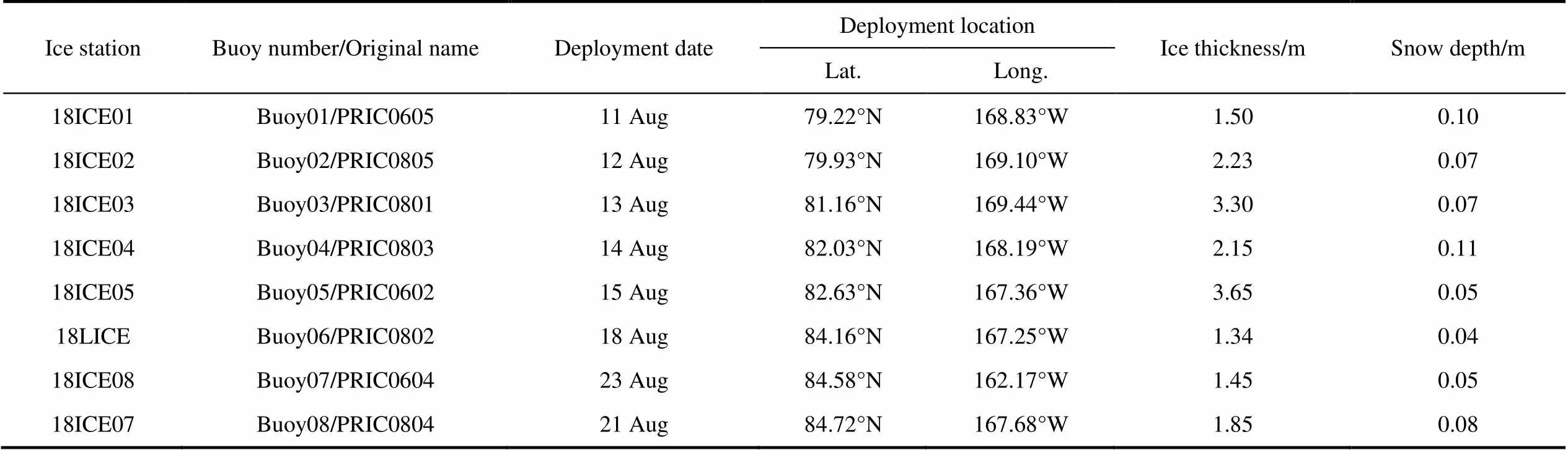
Table 1 Details of buoys and buoy deployment

Under the effect of the clockwise BG, all the buoys used in this study drifted eastward and slightly southward until mid-December 2018, with the trajectories being approximately parallel (Figure 1). Between mid-December 2018 and mid-March 2019, trajectories turned northeastward with the northeast drift being more accentuated for the buoys in the north. Between mid-December and mid-March, the three northernmost buoys gradually moved away from the BG system and merged into the Transpolar Drift Stream (TDS) system. The five buoys in the south remained in the BG system, and drifted clockwise again in summer 2019.

Figure 1 Drifting trajectories of the buoys superposed over the sea ice concentration on 1 August 2018. Also shown are the monthly sea ice edges of August 2018 (brown line) and August 2019 (gray line).

2.2 Determination of atmospheric anomalies

We examined the large-scale atmospheric circulation and the meteorological conditions along buoy trajectories. To quantify the effect of the atmospheric circulation on sea ice motion, we calculated the seasonal Arctic Oscillation (AO) and Dipole Anomaly (DA) indices, which are defined as the first and second modes of the empirical orthogonal function applied to the Sea Level Pressure (SLP) north of 70°N from the NCEP/NCAR (the National Centers for Environmental Prediction and the National Center for Atmospheric Research) reanalysis (Wang et al., 2009). This definition is based on SLP in the far north, while some other definitions are based on SLP from almost the entire Northern Hemisphere, such as poleward of 20°N (Thompson and Wallace, 2000). We argue that, a definition that is based on SLP in the far north is more appropriate for studies on the atmospheric circulation in the Arctic region (Wang et al., 2009). The AO mainly reflects the influence of the atmosphere on the zonal circulation intensity (Thompson and Wallace, 2000; Zhang et al., 2021). Positive AO promotes cyclonic wind and sea ice circulation, and the BG system retracts and weakens (Wang and Ikeda, 2000). The DA is mainly a meridional forcing; it promotes northward drift of sea ice in the BG system (Wang et al., 2009; Lei et al., 2019). In the BG region, mean sea ice motion is clockwise because of the generally anticyclonic atmospheric circulation. The boundary and strength of the BG are mainly regulated by the Beaufort High (BH; Proshutinsky et al., 2009; Lei et al., 2019). Because all the buoys were deployed in the BG region, we calculated the BH index as a benchmark. Following Moore et al. (2018), we calculated the BH index using the anomaly of SLP across the region of 75°N–85°N and 170°E–150°W from ERA 5 reanalysis data. We used the seasonal atmospheric circulation indices of AO, DA, and BH to identify the anomalies in atmospheric circulation during the study period of September 2018 to August 2019 relative to 1979–2019 climatology.

The hourly air temperature at 2 m (T2m) and wind speed at 10 m (W10m) from the ERA 5 reanalysis data provided by the European Centre for Medium-Range Weather Forecasts (ECMWF; Hersbach et al., 2020) were bilinearly interpolated onto buoy trajectories for September 2018 to August 2019 and for the 40 years after 1979. The latter period was used as the long-term reference. Arctic sea ice extent decreased considerably between 2010 and 2019. Thus, we also calculated mean near-surface meteorological conditions for 2010–2019. We identified the anomalies of near-surface meteorological conditions during the study period relative to 1979–2019 and 2010–2019 means, respectively. The long-term trend of monthly T2m along the trajectory of each buoy was also identified to assess the potential impacts of long-term changes on meteorological anomalies during the study period.

2.3 Determination of sea ice anomalies

We used satellite remote sensing products to determine the anomalies of sea ice conditions along buoy trajectories. The daily products of sea ice concentration derived from the Nimbus-7 Scanning Multichannel Microwave Radiometer (SMMR) and its successors (SSM/I and SSMIS) (Fetterer et al., 2017), as well as the Motion Vectors Version 4 dataset (Tschudi et al., 2019) provided by the National Snow and Ice Data Center (NSIDC), were used to estimate anomalies of ice concentration and drift speed. Using ERA 5 reanalysis W10m and satellite sea ice motion products, we calculated the speed ratio between sea ice and wind. This parameter is a measure of sea ice response to wind forcing (Vihma et al., 1996; Zhang et al., 2021), and we used it to identify the spatial and seasonal variations in sea ice sensitivity to wind forcing and their anomalies during the study period. Several assessments indicate that the accuracy of passive microwave sea ice concentration is approximately 5% in the freezing season, and 10%–20% in the melt season (Peng et al., 2013; Beitsch et al., 2015). Comparisons between buoy data and the NSIDC product show that the NSIDC product underestimated daily sea ice drift speed with relative errors of −0.6% to −2.0% for the freezing season and −7.2% to −10.0% for the melt season(Gui et al., 2020). Because this remote sensing sea ice motion products are available throughout the year, they have been used to identify long-term changes and anomalies of sea ice conditions (e.g., Krumpen et al., 2021; Zhang et al., 2021).

We used the weekly merged CryoSat2-SMOS sea ice thickness product provided by the Alfred Wegener Institute (Ricker et al., 2017) to estimate anomalies of ice thickness in the freezing season. The data are available for October to April from 2010 to present day. The product has a spatial resolution of 25 km, and should include thickness changes caused by thermodynamic growth and sea ice deformation. Ice growth rate estimated from CryoSat2-SMOS data was approximately 1.7 times that derived from data collected by 11 SIMBA buoys deployed during MOSAiC; this discrepancy may indicate potential overestimation of ice growth in the CryoSat2-SMOS product and the inability of the buoys to capture ice thickness increases caused by deformation (Lei et al., 2022). Ice growth rate estimated from CryoSat2-SMOS data was 118% that derived from airborne electromagnetic induction sounding (von Albedyll et al., 2021; Lei et al., 2022). The temporal coverage of laser altimetry data from ICESat-2 (e.g., Koo et al., 2021) is relatively short. Radar altimetry data have relatively low resolution and accuracy compared to the laser altimetry, but they are the only data that can be used to identify changes in sea ice thickness over long periods.

We retrieved snow depth along buoy trajectories from the 7 GHz and 19 GHz channels of the Advanced Microwave Scanning Radiometer 2 (AMSR2) (Rostosky et al., 2018). The grid size of the snow depth data is 25 km. Currently, only snow depth in multi-year ice regions in March and April can be retrieved (Rostosky et al., 2018). The buoys were deployed in an area dominated by multi-year ice with relatively thick ice, which is favorable for snow depth retrievals. We compared the snow depth in March and April 2019 with the 7-year average from 2013 to 2019 to identify the anomalies during the study period. Snow depth data for the complete ice season are not available. For Arctic sea ice, snow generally starts to melt in May (Lei et al., 2022); therefore, snow depths in March and April represent annual maxima. The uncertainty for AMSR2 snow depth data on multi-year ice was estimated to be 8 cm based on comparisons with in situ snow measurements along the MOSAiC transect (Krumpen et al., 2021).

To identify the ice surface melt onset using the dataset from passive microwave observations (Markus et al., 2009), we only used the continuous melt onset, which is defined as the date after which ice surface melting persists. This is because the continuous melt onset is more stable than the first date with ice surface melt. The spatial resolution of the ice surface melt onset dataset is 25 km. We only used the data from 1988 to 2019, although it is available since 1979, because there are some data gaps in the study area prior to 1988. We did not consider the index of ice surface freezing onset because ice surface freezing onset occurred before or after the beginning of the study period (1 September), which led to the difficulties to match the index to the buoy trajectories.

All data, except for ice melt onset, were linearly interpolated to each buoy location for the time on which the buoy was at that location. For each buoy trajectory, we retrieved ice surface melt onset from the passive microwave dataset; from the dates that buoy data were available, we selected the date that was closest to the passive microwave melt onset and defined it as the surface melt onset. No evidence shows that the deviation of satellite products for the above sea ice parameters reveals yearly change. Therefore, we believe that the uncertainties of the data, though not negligible, will not affect the identified sea ice anomalies.

3 Results and discussions

3.1 Atmospheric circulation anomalies

In autumn 2018, AO, DA, and BH were near neutral, and deviations from the 1979–2019 climatology were less than one standard deviation. There was a relatively weak high-pressure system over the southern Beaufort Sea, which resulted in buoy trajectories and wind vector anomalies at buoy locations that were almost parallel to the latitude lines in this season (Figure 2a). In the winter of 2018–2019, an anomalously high (positive) DA was the most distinct characteristic of the atmospheric circulation. While, the BH was anomalously low (negative). The 2018–2019 DA index was the second highest between 1979 and 2019; the 2018–2019 BH index had the fourth lowest magnitude between 1979 and 2019. In the winter of 2018–2019, there was a relatively strong low-pressure system over the north of the Laptev–East Siberia seas, which, together with a high-pressure system over the Canadian Arctic Archipelago, resulted in the extreme positive DA. The wind vector anomalies at buoy locations were almost parallel to the northern shore of the Canadian Arctic Archipelago. This SLP pattern likely caused a temporary reversal in the BG system, which led to northward advection of sea ice and the sea ice entering the TDS system in mid-December 2018. Figures 1 and 2b show the three buoys in the north starting to move away from the BG system at this time. The influence of this SLP pattern on the five buoys in the south was relatively weak. In spring 2019, the DA index was the sixth highest between 1979 and 2019, and was weaker than the DA in the winter of 2018–2019 (Table 2). As a result, the buoys in the north moved further away from the BG system. However, the net ice advection in spring was much smaller than that in winter because spring wind forcing was close to that of the 1979–2019 climatological mean (Figure 2c). In summer 2019, the AO was anomalously low (negative), while the BH was anomalously high (positive), with a high-pressure system dominating the central Arctic Ocean. Relative to the 1979–2019 climatology, wind vectors at buoy locations were distinctly anticyclonic (Figure 2d). This atmospheric circulation pattern considerably strengthened the clockwise circulation of the sea ice. Thus, the five buoys in the south resumed their clockwise movement southward.

Figure 2 Seasonal anomalies of sea level pressure (SLP) and wind vector over the Arctic Ocean during the ice season of 2018–2019 relative to the 1979–2019 climatology. Also shown are buoy trajectories for each season.

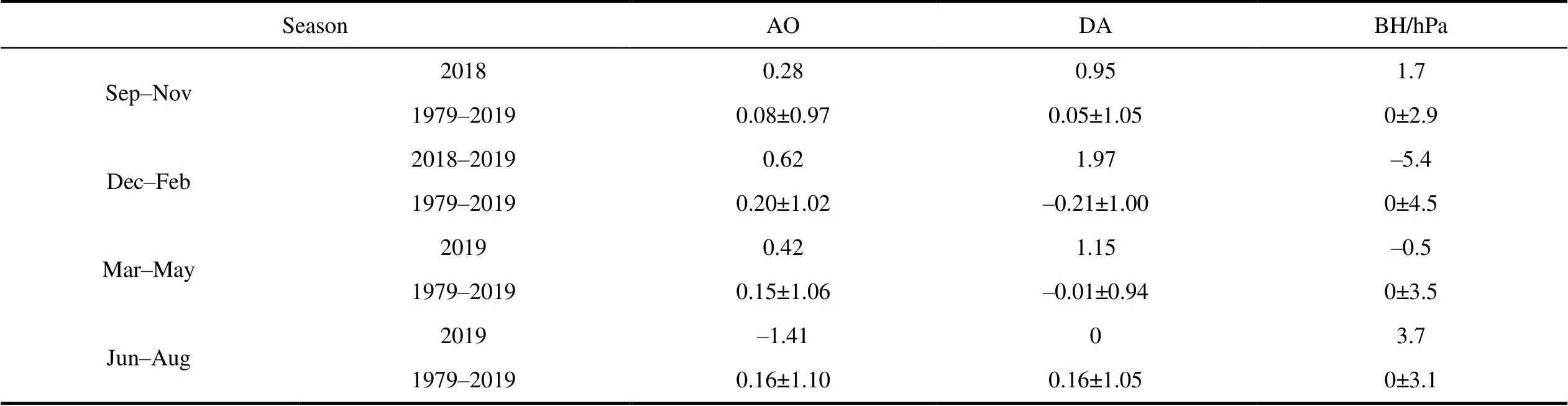
Table 2 Seasonal atmospheric circulation indices for the ice season of 2018–2019 and climatological means from 1979 to 2019

Sea ice advection in the western Arctic Ocean is influenced by the AO, BH, and DA. The BH is the index that describes the BG system. Therefore, its influence on sea ice circulation is considerably stronger than that of the AO. Positive DA led to the northward drift of the buoys deployed north of 84°N. Thus, the deployment sites of the three northernmost buoys can be considered as the boundary between the BG and the TDS systems. Whether the buoys and their ice floes were finally captured by the BG or merged into the TDS largely depended on the DA. Although, the overall direction of sea ice advection was mainly determined by the large-scale atmospheric circulation, sea ice drift is a combination of general advection and irregular motions and cycles at smaller scales. These small-scale movements are mainly related to synoptic events, (e.g., cyclones; Haller et al., 2014) and the inertial oscillations of sea ice motion (e.g., Gimbert et al., 2012).

3.2 Anomalies in near-surface air temperature

We compared T2m in 2018–2019 along the buoy trajectories with 2009–2019 (past 10 years) and the 1979–2019 (past 40 years) means. In 2018–2019, T2m was relatively high between September and November when the sea ice began to freeze, and in April when there was increased sea ice deformation and lead formation (e.g., Qu et al., 2021). Synoptic-scale fluctuations could also influence seasonal variations. In winter, cyclones and other synoptic processes increased the near-surface temperature by up to 15 K (Figure 3). In 2018–2019, the warming events occurred in mid-December, mid-January, mid- February, early March, late March, and early April. Minimum air temperatures were also mainly related to synoptic events, which occurred on 10 January 2019 for the five buoys in the south (between −33.8 and −32.5 ℃), and on 17 March 2019 for the three northernmost buoys (between −34.9 and −33.6 ℃). For the annual average T2m between September and August of the following year, the 2018–2019 value exceeded the 1979–2019 value by 1.6± 0.4 K, and exceeded the 2009–2019 value by 0.7±0.3 K. This indicates that the T2m during the study period was closer to that in the past 10 years because of continuous Arctic warming. In addition, there was a significant negative correlation between the T2m anomaly of the study period and the latitude of buoy locations (R=0.80,<0.01). The T2m anomalies relative to the climatology were higher for the buoys that were closer to the southern MIZ.

We calculated the long-term trend of monthly T2m corresponding to each buoy to examine the influence of long-term changes on the meteorological anomalies identified in the buoy operation year (Figure 4). Generally, the positive trend in air temperature is more distinct and significant in the regions closer to the MIZ. Thus, the mean monthly latitude can explain the difference between T2m anomalies in the north and those in the south during the study period (Figure 3). As the MIZ of the Arctic Ocean retreats northward in summer (Strong and Rigor, 2013), significant autumn and winter warming is also expected to expand northward. We found significant positive trends of T2m in autumn, winter, and in April. At high latitudes north of 83°N, a significant positive trend of T2m was absent between December and August. However, at the lower latitudes that correspond to the locations of the southernmost buoy, the significant positive trend was maintained until May. The autumn T2m trend was 0.09 ± 0.03 K·a−1and the winter T2m trend was 0.08 ± 0.02 K·a−1. The autumn and winter trend of the near-surface air temperature north of 70°N between 1989 and 2008 from the ERA-Interim reanalysis was 1.6 K·(10 a)−1(Screen and Simmonds, 2010), which is comparable to our autumn T2m trend for the same period (1.64 ± 0.12 K·(10 a)−1) but is larger than our winter T2m trend (1.14 ± 0.44 K·(10 a)−1). This is likely because our study area is in a region with relatively heavy ice conditions, which has maintained nearly 100% ice cover in winter even in recent decades. The study area of Screen and Simmonds (2010) included large areas that were completely ice free in summer, especially in recent years; here, in winter, considerable heat transfer from the ice–ocean system to the lower atmosphere increases near-surface air temperature. This emphasizes that Lagrangian studies of anomalous meteorological conditions along buoy trajectories can capture variations in space and time more accurately to match the bouy measuremnets than Eulerian methodologies. There was no significant increase in near-surface air temperature in the Arctic Ocean in summer, mainly because of the absorption of atmospheric heat by melting ice. This mechanism, referred to as the effect of the water-ice bath by Overland (2009), can explain the seasonal variations of T2m anomalies during the study period.

Figure 3 a, Variations in near-surface air temperature at 2 m (T2m) from ERA 5 reanalysis data between September 2018 and August 2019 for the latitudes covered by buoy trajectories; b, 2018–2019 T2m anomalies relative to 1979–2019 means; c, 2018–2019 T2m anomalies relative to 2009–2019 means.

Figure 4 a, The long-term trends of monthly T2m along buoy trajectories; b, The square of their correlation coefficients. Purple circles indicate trends that are statistically significant at the 95% confidence level.

The T2m falls below the freezing point of seawater (−1.8 ℃) at all buoy locations in early September, and rise above the freezing point in June of the following year. Therefore, we defined the freezing season as September to June of the following year and the melt season as June to August. We calculated Freezing Degree Days (FDD)—the integral of T2m below the freezing point over the freezing season—and Thawing Degree Days (TDD)—the integral of T2m above the freezing point over the melt season. Figure 5 shows that 2018–2019 FDD was considerably lower than the FDD means of 1979–2019 and 2009–2019, with the largest differences at the lower latitudes because T2m anomalies in the freezing season were larger at lower latitudes. Variations in FDD were distinct from those in TDD. The difference between 2018–2019 TDD and the TDD means of 1979–2019 or 2009–2019 was smaller than that between 2018–2019 FDD and FDD means of 1979–2019 or 2009–2019. For TDD, the largest differences were observed at the higher latitudes. This is likely because: (1) Summer warming was weaker; (2) The water-ice bath effect was weaker at the higher latitudes; (3) Less energy was consumed to melt ice in summer at the high latitudes. The daily contribution to the difference between 2018–2019 TDD and 1979–2019 TDD was 0.06 ± 0.5 K, which was only 3% of the corresponding value for FDD (2.06 ± 0.57 K).

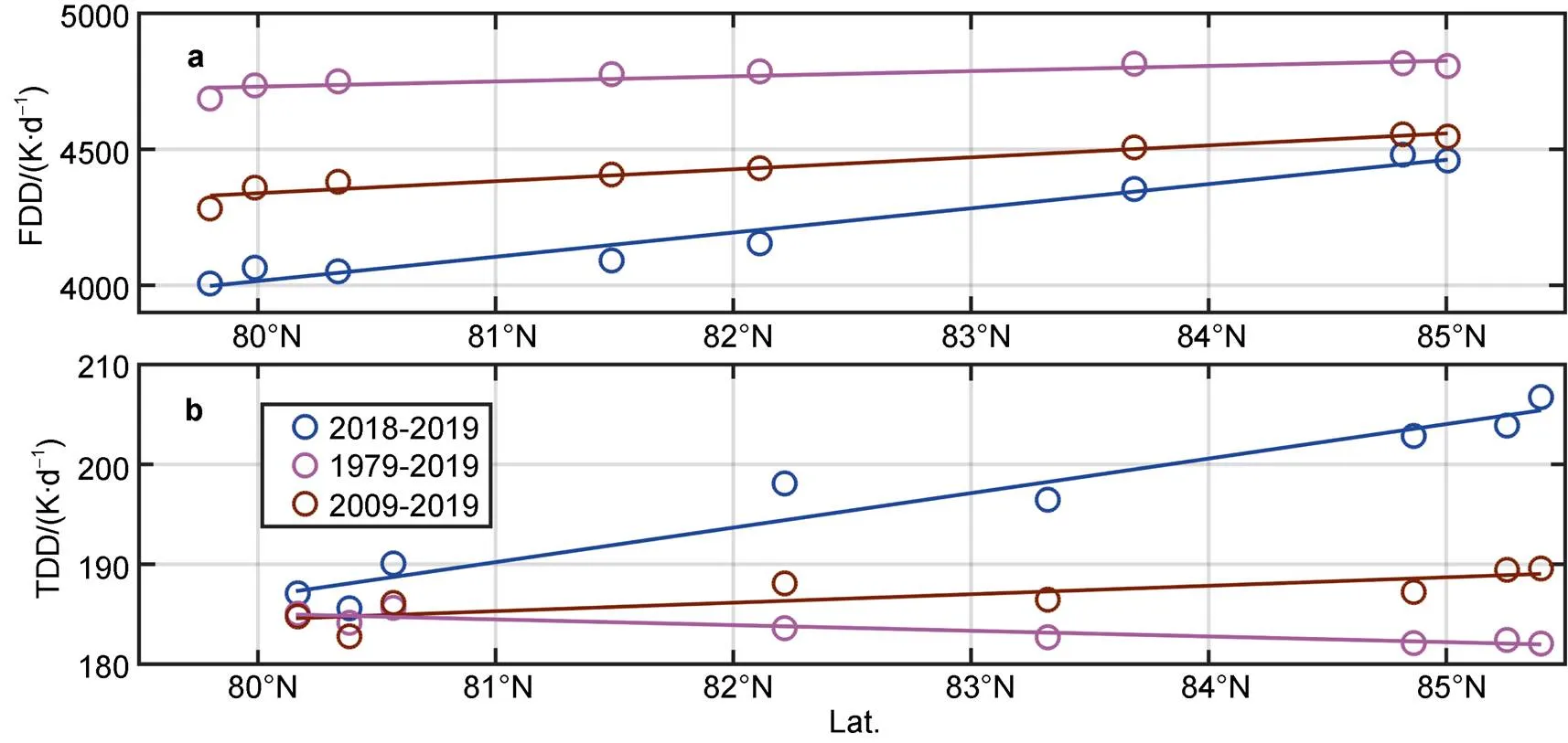
Figure 5 Cumulative Freezing Degree Days (FDD, a) for the freezing period (September to May) and Thawing Degree Days (TDD, b) for the melt period (June to August). All values were calculated for locations along buoy trajectories.

3.3 Anomalies in sea ice concentration

In the study area, the southern ice edge in August 2018 was at a lower latitude than that in August 2019 (Figure 1), suggesting that the ice conditions in summer 2018 were heavier than those in 2019. This can be partly attributed to the relatively cold near-surface air conditions over the study area in summer 2018. Summer (June to August) 925-hPa air temperatures in this year were below climatological means over coastal North America, the Chukchi Sea, the Beaufort Sea, and the Canadian Basin. Persistent cloudy and cool weather in June 2018 slowed sea ice melt in the western Arctic Ocean (Serreze et al., 2018). By late August 2018, there was still considerable ice in the Beaufort Sea near the coast. In August 2018, ice concentration at all buoy deployment sites exceeded 90% (Figure 6). Buoy deployment sites were far from the MIZ (defined as the region with ice concentration of less than 80%). By the end of the study period, all the buoys were still in the PIZ where ice concentration was close to 100%. The southernmost buoy was approximately 400 km from the ice edge. Along buoy trajectories, ice concentration in 2018–2019 was generally comparable to the 1979–2019 mean ice concentration, except for the southernmost buoy trajectories, where, in early autumn, ice concentration in 2018–2019 was slightly lower than 1979–2019 mean.

Along all buoy trajectories, in early autumn, sea ice condition in 2018 was heavier than that in 2009–2019, especially for the region south of 82°N; ice concentrations reached nearly 100% by mid-October; in mid-May 2019, ice concentration started to drop below 95% occasionally (Figure 6). This is likely related to increased sea ice deformation (Lei et al., 2020) and frequent occurrence of leads in spring (e.g., Qu et al., 2021).

3.4 Anomalies in sea ice thickness and snow depth

When the buoys were deployed in mid-August 2018, we measured the ice thickness at the deployment sites, which was averaged at 2.18 ± 0.86 m (Table 1). After deployment, the buoys recorded ice thickness decreases of around 0.05–0.25 m by early October 2018 (not shown). Ice thickness from the CryoSat2-SMOS product in early October was 2.00 ± 0.37 m. Thus, ice thickness at the deployment sites can be considered to be spatially representative at the scale of the CryoSat2-SMOS grid (～25 km). This is because the deployment sites included the level ice and ice ridges, which were similar to the composition of ice categories within the footprints of satellite observations.

Figure 7 shows that ice thickness increased considerably from south to north along buoy trajectories in both 2018–2019 and 2010–2019. This spatial pattern in ice thickness weakened from autumn to spring because there was similar atmospheric forcing, such as T2m (Figure 3) from south to north, and the growth rate of the thin ice in the south was higher than that of the thick ice in the north. Ice thickness in October 2018 was slightly higher than the 2010–2019 average, especially in the north (Figure 7a). This small deviation had almost completely disappeared by mid-December (Figure 7b). After mid-December, ice growth rate during the study year was almost consistent with that of 2010–2019. The average ice thickness at the buoy sites increased by 0.96 m between October 2018 and April 2019; ice growth rate was 0.55 cm·d−1, which was slightly lower than the 2010–2019 average (0.67 cm·d−1). Ice growth rate from the CryoSat2-SMOS product includes the contributions of thermodynamic growth and deformation of sea ice. The T2m between October 2018 and April 2019 was slightly higher than that in 2010–2019 by 0.5 K. Thus, difference in T2m and potential year-to-year differences in sea ice dynamics could have led to the difference in ice growth rate.

Generally, the ice thickness measurements that were obtained at the beginning of the study period and the spatial and seasonal variations of ice thickness and ice growth rate during the study period were representative of the corresponding values from the past 10 years.

Figure 6 The same as Figure 3, but for sea ice concentration.

Figure 7 a, Monthly sea ice thickness interpolated to buoy locations from October 2018 to April 2019; b, 2010–2019 mean monthly sea ice thickness; c, Mean and standard deviation of sea ice thickness from 2018–2019 and 2010–2019.

Snow depth in the south was smaller than that in the north, with the maximum deviation of around 0.15 m occurring in March–April 2019 (Figure 8a). This difference can be considered robust because it exceeded the potential uncertainty of the snow depth product (5–10 cm; Krumpen et al., 2021). In 2019, the snow depth in the north exceeded the 2012–2019 average, and the snow depth in the south was below the 2012–2019 average (Figure 8b). Between March and April, mean snow depth in 2019 was comparable to that in 2012–2019, with a deviation of less than 0.02 m. Between early and mid-March, snow accumulation in 2019 was higher than the 2012–2019 average (Figure 8c). In both 2019 and 2012–2019, snow depth remained relatively stable between mid-March and mid-April, except for short-term fluctuations due to synoptic processes. Between 15 March and 10 April, average snow depth was 0.31 m in 2019 and 0.30 m in 2012–2019, respectively. These values can be considered as annual maxima because snow started melting after 10 April, especially for the buoys in the south (Figure 8a). These results indicate that the AMSR2 product can reliably estimate snow depth in the study area during the period between the time with annual maximum snow depth and snow melt onset. At the end of April 2019, the contribution of snow to the mass balance of snow-covered sea ice was derived usings×s/i/(s×s/i+i), wheresandiare snow and ice thicknesses, andsandiare snow and ice densities, and were assumed to be 300 and 900 kg·m−3, respectively. The contribution of snow was 3.1% in 2019 and 3.2% in 2012–2019, respectively. Thus, annual maximum snow depth, the first day of snow depth decrease, and the contribution of snow to sea ice mass balance in early spring 2019 were very close to the corresponding values from 2012–2019.

Figure 8 Variations in snow depth for the latitudes covered by buoy trajectories between 1 March and 30 April in 2019 (a), 2012–2019 (b), and their spatial averages (c).

3.5 Anomalies in wind and sea ice drift speeds

Figure 9a shows absence of notable seasonal or spatial variations in wind speed in 2018–2019. Episodic increases in wind speed were mainly related to synoptic events, such as storms. Most heavy storms occurred during late September and late December 2018, with the maximum wind speed reaching approximately 15 m·s−1. Although storm events are reasonably reproduced in the hourly wind data of the ERA 5 reanalysis, ERA 5 wind speeds are often underestimates of wind speeds during storms (e.g., Rinke et al., 2021), which results in the difficulties to capture instantaneous wind speed increases. Thus, we believe that the extreme wind speed values from our analysis are underestimates. The annual average wind speed in 2018–2019 was 4.83±0.13 m·s−1, which was slightly lower than that in 1979–2019 (5.27±0.03 m·s−1) and in 2009–2019 (5.21±0.03 m·s−1). Thus, the wind forcing along the buoy trajectories during 2018–2019 can be considered normal relative to 1979–2019 or 2009–2019 climatology. The largest anomalies in 2018–2019 wind speed relative to climatology were found in December 2018 (positive anomaly) and January 2019 (negative anomaly).

Wind forcing is the main driver of sea ice motion. Sea ice drift speed increased (Figure 10a) in response to extreme wind speeds (Figure 9a). However, the temporal and spatial variations in ice speed also differed from those of wind forcing. Ice speed decreased gradually from autumn to winter and increased again as summer approached. In autumn, early winter, and summer, speeds of the buoys in the south were higher than those in the north. These characteristics were more pronounced in 2018–2019 and 2009–2019 than in 1979–2019 because of the gradual increase in sea ice mobility.

To quantify the temporal and spatial changes in sea ice mobility, we used remote sensing sea ice motion products and reanalysis wind speeds to calculate the ratio between ice and wind speeds (Figure 11). This ratio ranged from close to 0 to around 5% (Figure 11a). Similar to ice speed, the ratio was higher in autumn, early winter, summer, and during storms, and lower in late winter, spring, or during periods with mild wind forcing. Spatial means showed clear seasonal variations (Figure 11d). For 1979–2019 and 2009–2019, the ratio decreased gradually from September to late March, and increased again from April to August. The ratio in late August remained lower than that in autumn of the previous year.

Figure 9 The same as Figure 3, but for wind speed.

Figure 10 The same as Figure 3, but for sea ice drift speed.

We believe that the seasonal variations of the speed ratio correspond to variations in the compactness of the ice field, which are related to ice concentration, thickness, and temperature (Hibler, 1979). In the north, there were no seasonal variations in ice concentration because the buoys remained in the PIZ during the whole study period. However, in the south, ice concentration increased rapidly in September (Figure 4). The ice thickness increased steadily from October to mid-April for all buoy sites (Figure 7). Seasonal variations in near-surface air temperature (Figure 3) were accompanied by considerable changes in the bulk average ice temperature. The bulk average ice temperature decreased from September to March or April to its annual minimum value, and graduallyincreased with increasing air temperature. Seasonal variations in the above parameters shape the temporal variations in the compactness of the ice cover and the ice–wind speed ratio. Moverover, the annual cycle of the ice–wind speed ratio is asymmetrical; the value in August is below that in September of the previous year (Figure 11d). This is likely related to spatial variations in ice conditions in the study area. After deployment, the buoys drifted eastward and approached the Canadian Arctic Archipelago; the buoys, especially those in the north, were in some of the heaviest ice conditions in the Arctic Ocean (Figure 1).

The 2018–2019 and 2009–2019 speed ratios were considerably larger than the 1979–2019 ratio, especially for September and October. For September, the speed ratios in 2018 and 2009–2019 were close to 2%, implying that the sea ice field has been relatively loose and the ice has been close to free drift in September in recent years (Leppäranta, 2011). This was because the relatively high ice temperature and low ice concentration in September reduced the compactness of the ice cover. We derived the ice–wind speed ratio using the daily sea ice motion product, which has a low sampling frequency and ignores intradayoscillations of sea ice motion (Haller et al., 2014). As a result, sea ice drift speed and ice–wind speed ratio may be underestimated by 30% in September and by around 20% in winter (Lei et al., 2021).Thus, the seasonal variations of the speed ratio, as well as the difference of the speed ratio in recent years against those in 1979–2019 shown in Figure 11d are expected to be underestimated.

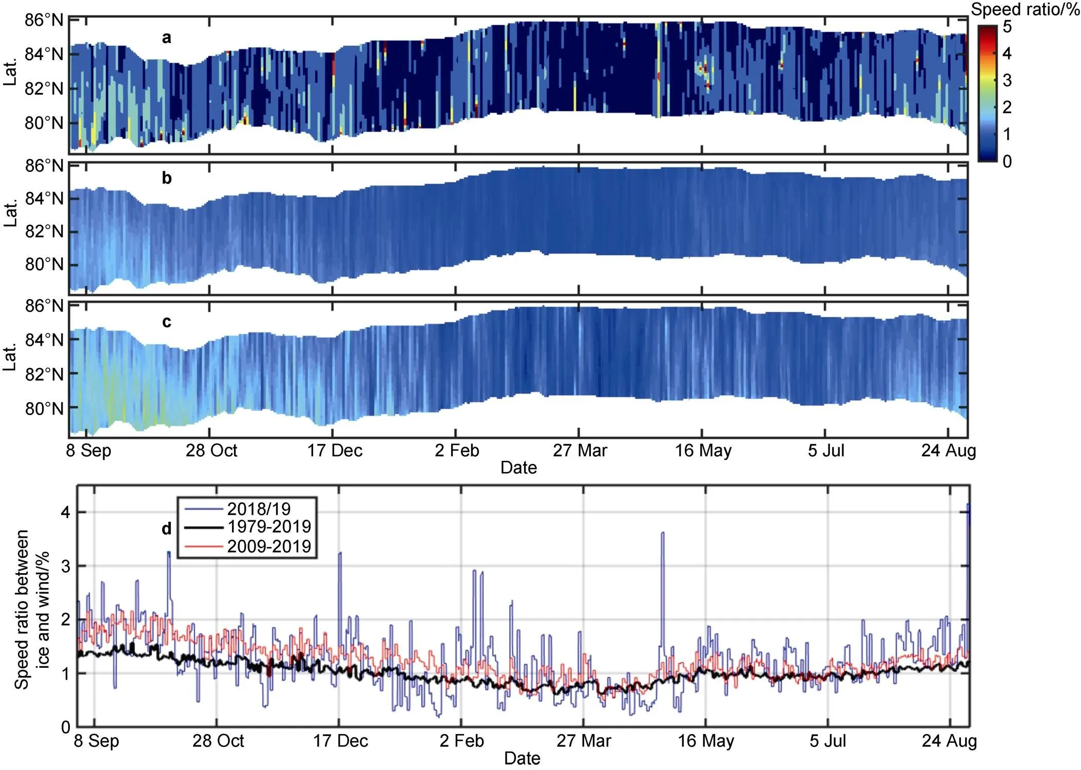
Figure 11 Variations in the ratio between sea ice and wind speeds (a) between September 2018 and August 2019 for the latitudes covered by buoy trajectories, (b) between September and August of the following year for 1979–2019, (c) between September and August of the following year for 2009–2019, and (d) seasonal variations in spatial means of the ice–wind speed ratio for 2018–2019, 1979–2019, and 2009–2019.

3.6 Anomalies in sea ice surface melt onset

In 2019, melt onset was between 13 June and 7 July (Table 3); the average was 25 June, which was comparable with the average of 1988–2019 (22 June). The melt onset was approximately 1–2 months after the first day of snow depth decrease (Figure 8). This is likely because the early stages of snow depth decrease are caused by evaporation, erosion, or metamorphism, and surface water content remains relatively stable. The appearance of surface water is the main criterion that is used to identify surface melt from passive microwave data (Markus et al., 2009). For all buoys, the surface melt onset in 2019 was within (or close to) one standard deviation of the 1988–2019 average. This implies that the ice surface melt onset in 2019 can be considered normal relative to 1988–2019. The main reasons include: (1) the change in the ice surface melt onset is smaller than that in the ice surface freezing onset, especially in the region with heavy ice conditions around the Canadian Arctic Archipelago (Markus et al., 2009); (2) the long-term trends of near-surface air temperature along all buoy trajectories were statistically insignificant in early summer (Figure 4); and (3) factors (1) and (2) resulted in surface melt onsets that showed no statistically significant trends between 1988 and 2019.

However, the spatial variations in surface melt onset in 2019 were different from those in 1988–2019. The surface melt onset was delayed from south to north (R=0.64,<0.05) for the 1988–2019 data. However, melt onset in the north was earlier than that in the south, with the trend being statistically significant at the 99% confidence level (R= 0.72) in 2019. This was likely related to the anomalous atmospheric circulation in June 2019 because melt onset is significantly correlated to the average air temperature over one month prior to melt onset. In June, there was a high-pressure system over the North American side of the Arctic at sea level, which drew in relatively cold air from the Beaufort Sea along the coast of Canada, and resulted in a lower near-surface air temperature in the south and a higher temperature in the north of the study region (Figure 12). This meridional gradient of near-surface air temperature in June 2019 was different from the situation in 1988–2019, and caused melt onset to occur later in the south than in the north in 2019.

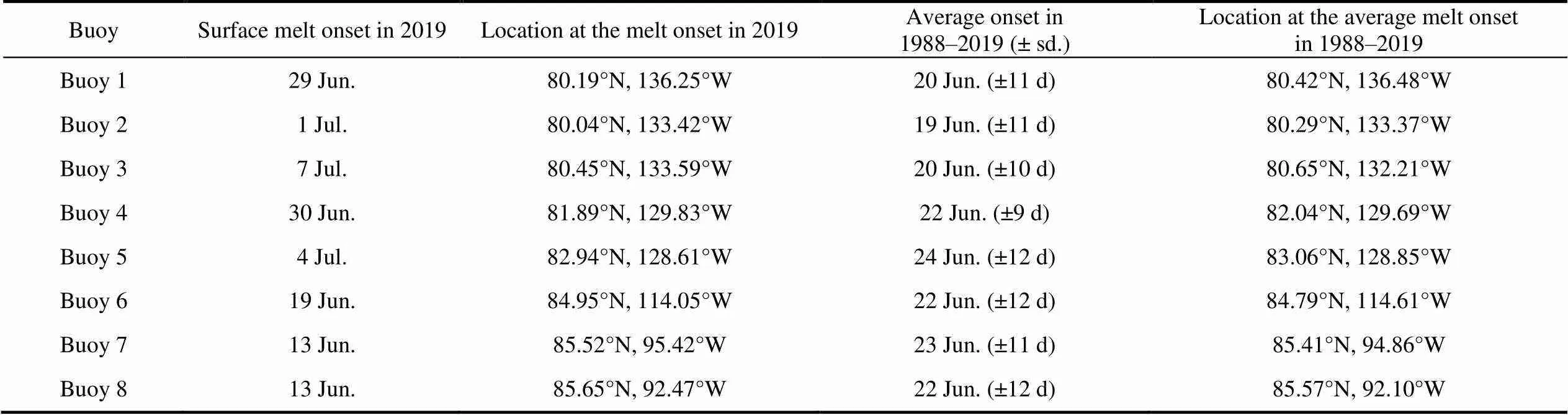
Table 3 Ice surface melt onset in 2019, average melt onset for 1988–2019, and buoy locations at melt onset

At the buoy locations at melt onset in 2019, there was a southward wind vector anomaly in June 2019 relative to the 1988–2019 average (Figure 12). This anomaly drew relatively cold air from the north into the study area and also resulted in higher air temperatures in the north and lower temperatures in the south. This wind pattern stabilizes the MIZ, and prevents it from retreating to the north. As a result, sea ice concentration at buoy locations in summer 2019 was comparable to that of the climatology (Figure 6).

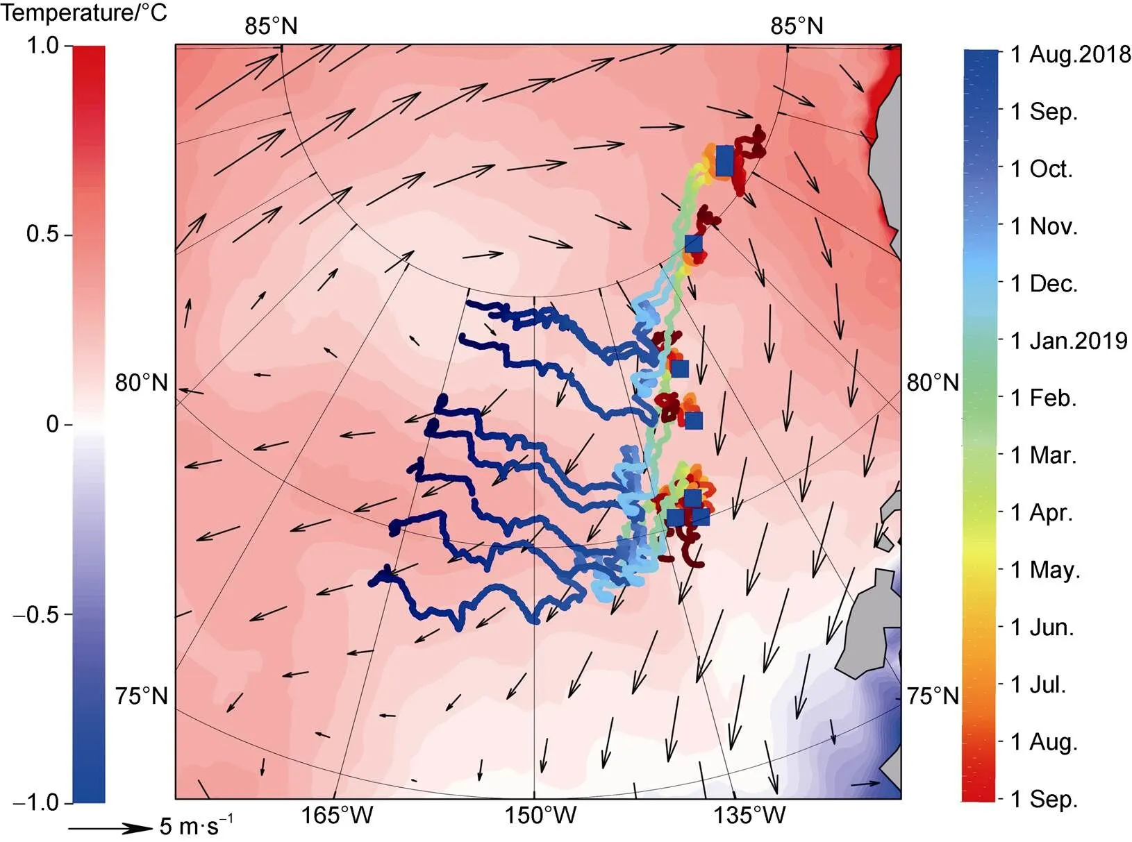
Figure 12 Drift trajectories of the buoys and buoy locations (blue squares) at ice surface melt onset in 2019. Also shown are the anomalies of the T2m and wind vectors in the study area in June 2019 relative to the 1988–2019 climatology.

4 Conclusions and outlook

Eight sea ice mass balance buoys were deployed in the western Arctic Ocean in August 2018. They were deployed in the sector of 160°W–170°W and at nearly regular intervals between 79.2°N and 84.7°N. This deployment strategy was designed to facilitate the characterization of the meridional differences in sea ice physical processes and responses to atmospheric forcing. After deployment, the buoys drifted eastward almost in parallel. In December 2018, the buoy array began to drift in separate directions. Three buoys in the north gradually drifted to the northeast and merged into the TDS system, while the other five buoys in the south remained within the BG system. This ice advection pattern can be related to a strong positive DA and an extreme negative BH. We used reanalysis data and satellite remote sensing sea ice products to identify the anomalies in the atmospheric forcing and ice conditions along the buoy trajectories during the year of buoy operation (2018–2019) and investigated possible causes of the anomalies.

The long-term increase in near-surface air temperature resulted in lower FDD in the freezing season (September to May) and higher TDD in the melt season (June to August) during the ice season of 2018–2019 relative to the 1979–2019 climatology. Because of differences in the coupling between atmosphere and sea ice during the freezing and melt seasons, FDD decrease was larger in the MIZ, while TDD increase was larger in the PIZ. We speculate that the heat uptake from the ice–ocean system during the freezing season was larger in the MIZ than in PIZ because of faster ice growth in the MIZ; while in the melt season, the rapid ice melt in the MIZ would absorb more heat and offset most of the heat released from the ocean to the atmosphere.

In the southern part of the study area in autumn, ice concentration in the 2018–2019 ice season was larger than mean ice concentration from the past 10 years, and was comparable to the 1979–2019 climatology. We found no ice concentration anomalies in other seasons. Both the ice thickness during the freezing season and the snow depth in March–April of the 2018–2019 ice season can be considered normal relative to the means of the past 7 or 9 years. Ice thickness at the buoy deployment sites was representative of the thickness of the ice inside the footprint of the satellites that generate remote sensing sea ice data. Therefore, we conclude that the sites selected for buoy deployment were suitable for the study of sea ice mass balance. Although the annual average wind speed in 2018–2019 was slightly lower than that in 1979–2019 and that in 2009–2019, the ice speed and its ratio to the wind speed were anomalously high for almost all seasons during the study year, except for March–May when ice field compactness was expected to be at its annual maximum. Thus, the seasonal changes and spatial differences between the MIZ and PIZ in the ice speed and its ratio to wind speed are expected to increase with the loss of Arctic sea ice. In 2019, and averaged over all the buoys, ice surface melt appeared on 25 June, which can also be considered normal relative to the 1988–2019 climatology. However, spatial variations of ice surface melt onset in 2019 differed from those in 1988–2019. Because a high-pressure atmospheric system prevailed over the Canadian coast of the Beaufort Sea in June 2019, ice surface melt onset in low latitudes occurred later in 2019 than in 1988–2019.

In addition to seasonal changes, the meteorological and sea ice anomalies were influenced by spatial differences. The buoys drifted eastward and entered the region with the heaviest ice conditions in the Arctic Ocean. The ice conditions at the buoy locations in the summer of the second year of the study were different from those at the buoy locations in early September of the first year. In this study, we identified meteorological and sea ice anomalies along the drifting trajectories of buoys in 2018–2019. Drifting trajectories of floes with the same starting points are expected to change every year because of variations in the atmospheric circulation and ice conditions (Lei et al., 2019). In the same year, the meteorological and ice conditions along different trajectories would also change (Lei et al., 2019). Therefore, the year-to-year change in sea ice drift trajectories will also determine the anomalies in meteorological and ice conditions retrieved along the trajectories. In future studies, we will use the buoy deployment sites as starting points and retrieve drifting trajectories using satellite remote sensing sea ice motion products for different years to identify the impact of the changes in atmospheric circulation and drifting trajectories on meteorological and ice anomalies. Moreover, we can combine the observation data from IMB, reanalysis data, and sea ice thermodynamic models to simulate the year-to-year changes in sea ice mass balance to identify the mechanisms whereby changes in climate and atmospheric circulation influence sea ice mass balance processes.

In summer and autumn 2018, in addition to the IMB deployed during the CHINARE cruise in the Arctic Ocean, some buoys were deployed in the northern East Siberian Sea during the T-ICE cruise (Lei et al., 2021). Therefore, by combining the observation data from IMB that were deployed on different cruises, we can further study sea ice mass balance processes and their response to atmospheric forcing and identify the differences between the western Arctic Ocean and other regions of the Arctic Ocean.

This work was supported by grants from the National Key Research and Development Program (Grant no. 2021YFC2803304) and the National Natural Science Foundation of China (Grant nos. 41976219 and 42106231). The SMMR and SSMIS ice concentration and ice motion products and the monthly Arctic sea ice index were provided by the NSIDC. The passive microwave satellite observations of ice surface melt onset are available at the https://earth.gsfc. nasa.gov/cryo. The gridded CryoSat/SMOS data sets are available via ftp://ftp.awi.de/sea_ice/product/cryosat2_smos/v203/nh/. Snow depth data are available from the PANGAEA. Atmospheric reanalysis data were obtained from the European Centre for Medium Range Weather Forecasts and the National Centers for Environmental Prediction/National Center for Atmospheric Research. We thank the Editors-in-Chief, Associate Editor, and two anonymous reviewers for their helpful feedback, which substantially improved the manuscript.

Behrendt A, Dierking W, Witte H. 2015. Thermodynamic sea ice growth in the central Weddell Sea, observed in upward-looking sonar data. J Geophys Res Oceans, 120(3): 2270-2286, doi:10.1002/2014jc010408.

Beitsch A, Kern S, Kaleschke L. 2015. Comparison of SSM/I and AMSR-E sea ice concentrations with ASPeCt ship observations around Antarctica. IEEE Trans Geosci Remote Sens, 53(4): 1985-1996, doi:10.1109/TGRS.2014.2351497.

Comiso J C, Meier W N, Gersten R. 2017. Variability and trends in the Arctic sea ice cover: results from different techniques. J Geophys Res Oceans, 122(8): 6883-6900, doi:10.1002/2017jc012768.

Fetterer F K, Knowles W N, Meier M, et al. 2017. Sea Ice Index, Version 3 [Data Set]. Boulder, Colorado USA. National Snow and Ice Data Center [2022-04-01], doi:10.7265/N5K072F8.

Gimbert F, Marsan D, Weiss J, et al. 2012. Sea ice inertial oscillations in the Arctic Basin. Cryosphere, 6(5): 1187-1201, doi:10.5194/tc-6- 1187-2012.

Gui D, Lei R, Pang X, et al. 2020. Validation of remote-sensing products of sea-ice motion: a case study in the western Arctic Ocean. J Glaciol, 66(259): 807-821, doi:10.1017/jog.2020.49.

Haller M, Brümmer B, Müller G. 2014. Atmosphere-ice forcing in the transpolar drift stream: results from the DAMOCLES ice-buoy campaigns 2007–2009. Cryosphere, 8(1): 275-288, doi:10.5194/tc-8- 275-2014.

Hersbach H, Bell B, Berrisford P, et al. 2020. The ERA5 global reanalysis. Q J Royal Meteorol Soc, 146(730): 1999-2049.

Hibler W D III. 1979. A dynamic thermodynamic sea ice model. J Phys Oceanogr, 9(4): 815-846, doi:10.1175/1520-0485(1979)009<0815: adtsim>2.0.co;2.

Jackson K, Wilkinson J, Maksym T, et al. 2013. A novel and low-cost sea ice mass balance buoy. J Atmos Ocean Technol, 30(11): 2676-2688, doi:10.1175/jtech-d-13-00058.1.

Koo Y, Lei R, Cheng Y, et al. 2021. Estimation of thermodynamic and dynamic contributions to sea ice growth in the Central Arctic using ICESat-2 and MOSAiC SIMBA buoy data. Remote Sens Environ, 267: 112730, doi:10.1016/j.rse.2021.112730.

Krumpen T, von Albedyll L, Goessling H F, et al. 2021. MOSAiC drift expedition from October 2019 to July 2020: sea ice conditions from space and comparison with previous years. Cryosphere, 15(8): 3897-3920, doi:10.5194/tc-15-3897-2021.

Lee S, Gong T, Feldstein S B, et al. 2017. Revisiting the cause of the 1989–2009 Arctic surface warming using the surface energy budget: downward infrared radiation dominates the surface fluxes. Geophys Res Lett, 44(20): 10654–10661, doi:10.1002/2017gl075375.

Lei R, Cheng B, Heil P, et al. 2018. Seasonal and interannual variations of sea ice mass balance from the central Arctic to the Greenland Sea. J Geophys Res Oceans, 123(4): 2422-2439, doi:10.1002/2017jc013548.

Lei R, Cheng B, Hoppmann M, et al. 2022. Seasonality and timing of sea ice mass balance and heat fluxes in the Arctic transpolar drift during 2019–2020. Elem Sci Anthropocene, 10(1): 000089, doi:10.1525/ elementa.2021.000089.

Lei R, Gui D, Hutchings J K, et al. 2019. Backward and forward drift trajectories of sea ice in the northwestern Arctic Ocean in response to changing atmospheric circulation. Int J Climatol, 39(11): 4372-4391, doi:10.1002/joc.6080.

Lei R, Gui D, Hutchings J K, et al. 2020. Annual cycles of sea ice motion and deformation derived from buoy measurements in the western Arctic Ocean over two ice seasons. J Geophys Res Oceans, 125(6): e2019JC015310, doi:10.1029/2019jc015310.

Lei R, Hoppmann M, Cheng B, et al. 2021. Seasonal changes in sea ice kinematics and deformation in the Pacific sector of the Arctic Ocean in 2018/19. Cryosphere, 15(3): 1321-1341, doi:10.5194/tc-15-1321- 2021.

Lei R, Tian-Kunze X, Li B, et al. 2017. Characterization of summer Arctic sea ice morphology in the 135°–175°W sector using multi-scale methods. Cold Reg Sci Technol, 133: 108-120, doi:10.1016/j. coldregions.2016.10.009.

Leppäranta M. 2011. The drift of sea ice, 2nd ed. Heidelberg: Springer-Praxis.

Markus T, Stroeve J C, Miller J. 2009. Recent changes in Arctic sea ice melt onset, freezeup, and melt season length. J Geophys Res, 114(C12): C12024, doi:10.1029/2009jc005436.

Moore G W K, Schweiger A, Zhang J, et al. 2018. Collapse of the 2017 winter Beaufort High: a response to thinning sea ice? Geophys Res Lett, 45(6): 2860-2869, doi:10.1002/2017GL076446.

Overland J E. 2009. Meteorology of the Beaufort Sea. J Geophys Res, 114: C00A07, doi:10.1029/2008jc004861.

Park K, Kang S M, Kim D, et al. 2018. Contrasting local and remote impacts of surface heating on polar warming and amplification. J Clim, 31(8): 3155-3166, doi:10.1175/jcli-d-17-0600.1.

Peng G, Meier W N, Scott D J, et al. 2013. A long-term and reproducible passive microwave sea ice concentration data record for climate studies and monitoring. Earth Syst Sci Data, 5: 311-318, doi:10.5194/essd-5-311-2013.

Proshutinsky A Y, Johnson M A. 1997. Two circulation regimes of the wind-driven Arctic Ocean. J Geophys Res, 102(C6): 12493-12514, doi:10.1029/97jc00738.

Proshutinsky A, Krishfield R, Timmermans M L, et al. 2009. Beaufort Gyre freshwater reservoir: state and variability from observations. J Geophys Res, 114: C00A10, doi:10.1029/2008jc005104.

Provost C, Sennéchael N, Miguet J, et al. 2017. Observations of flooding and snow-ice formation in a thinner Arctic sea-ice regime during the N-ICE 2015 campaign: influence of basal ice melt and storms. J Geophys Res Oceans, 122(9): 7115-7134, doi:10.1002/2016jc012011.

Qu M, Pang X, Zhao X, et al. 2021. Spring leads in the Beaufort Sea and its interannual trend using Terra/MODIS thermal imagery. Remote Sens Environ, 256: 112342, doi:10.1016/j.rse.2021.112342.

Richter-Menge J A, Perovich D K, Elder B C, et al. 2006. Ice mass-balance buoys: a tool for measuring and attributing changes in the thickness of the Arctic sea-ice cover. Ann Glaciol, 44: 205-210, doi:10.3189/172756406781811727.

Ricker R, Hendricks S, Kaleschke L, et al. 2017. A weekly Arctic sea-ice thickness data record from merged CryoSat-2 and SMOS satellite data. Cryosphere, 11(4): 1607-1623, doi:10.5194/tc-11-1607-2017.

Rinke A, Cassano J J, Cassano E N, et al. 2021. Meteorological conditions during the MOSAiC expedition: normal or anomalous? Elem Sci Anthropocene, 9(1): 00023, doi: 10.1525/elementa.2021.00023.

Rostosky P, Spreen G, Farrell S L, et al. 2018. Snow depth retrieval on Arctic sea ice from passive microwave radiometers—improvements and extensions to multiyear ice using lower frequencies. J Geophys Res Oceans, 123(10): 7120-7138, doi:10.1029/2018jc014028.

Screen J A, Simmonds I. 2010. The central role of diminishing sea ice in recent Arctic temperature amplification. Nature, 464(7293): 1334-1337, doi:10.1038/nature09051.

Serreze M C, Stroeve J. 2015. Arctic sea ice trends, variability and implications for seasonal ice forecasting. Phil Trans R Soc A, 373(2045): 20140159, doi:10.1098/rsta.2014.0159.

Serreze M, Stroeve J, Bhatt U S, et al. Sea Ice Outlook: 2018 July Report (2018-07-20) [2022-03-30]. Turner-Bogren B, Wiggins H V and Stoudt S (eds). https: //www.arcus.org/sipn/sea-ice-outlook/2018/july.

Strong C, Rigor I G. 2013. Arctic marginal ice zone trending wider in summer and narrower in winter. Geophys Res Lett, 40(18): 4864-4868, doi:10.1002/grl.50928.

Thompson D W J, Wallace J M. 2000. Annular modes in the extratropical circulation. Part I: month-to-month variability. J Climate, 13(5): 1000-1016, doi:10.1175/1520-0442(2000)013< 1000: amitec>2.0.co;2.

Tschudi M, Meier W N, Stewart J S, et al. 2019. Polar Pathfinder Daily 25 km EASE-Grid Sea Ice Motion Vectors, Version 4 [Data Set]. Boulder, Colorado USA. NASA National Snow and Ice Data Center Distributed Active Archive Center [2022-04-01]. doi:10.5067/INAWUWO7QH 7B.

Vihma T, Launiainen J, Uotila J. 1996. Weddell Sea ice drift: kinematics and wind forcing. J Geophys Res, 101(C8): 18279-18296, doi:10. 1029/96jc01441.

von Albedyll L, Hendricks S, Grodofzig R, et al. 2022. Thermodynamic and dynamic contributions to seasonal Arctic sea ice thickness distributions from airborne observations. Elem Sci Anthropocene, 10(1): 00074, doi:10.1525/elementa.2021.00074.

Wang J, Ikeda M. 2000. Arctic oscillation and Arctic sea-ice oscillation. Geophys Res Lett, 27(9):1287-1290.

Wang J, Zhang J, Watanabe E, et al. 2009. Is the Dipole Anomaly a major driver to record lows in Arctic summer sea ice extent? Geophys Res Lett, 36(5): L05706, doi:10.1029/2008gl036706.

Zhang F, Pang X, Lei R, et al. 2021. Arctic sea ice motion change and response to atmospheric forcing between 1979 and 2019. Int J Climatol, 42(3): 1854-1876, doi:10.1002/joc.7340.

10.13679/j.advps.2022.0005

27 April 2022;

25 July 2022;

30 August 2022

: Lei R B, Zhang F Y, Zhai M X. Meteorological and sea ice anomalies in the western Arctic Ocean during the 2018–2019 ice season: a Lagrangian study. Adv Polar Sci, 2022, 33(3): 204-219,doi:10.13679/j.advps.2022.0005

, ORCID: 0000-0001-8525-8622, E-mail: leiruibo@pric.org.cn