Population size and distribution of seabirds in the Cosmonaut Sea, Southern Ocean

LIN Zixuan, LIU Meijun, YAN Denghui, GAO Kai, LIU Xiangwan & DENG Wenhong

Population size and distribution of seabirds in the Cosmonaut Sea, Southern Ocean

LIN Zixuan, LIU Meijun, YAN Denghui, GAO Kai, LIU Xiangwan & DENG Wenhong*

Ministry of Education Key Laboratory for Biodiversity Science and Ecological Engineering, College of Life Sciences, Beijing Normal University, Beijing 100875, China

The Cosmonaut Sea is one of the less studied ecosystems in the Southern Hemisphere. Unlike other seas which were near to coastal regions, however, few studies exist on the top predators in this zone. From December 2019 to January 2020, a survey of seabirds was carried out on the board icebreaker R/Vin the Cosmonaut Sea and the Cooperation Sea. Twenty-three bird species were recorded. Antarctic petrel (), Antarctic prion (), and Arctic tern () were the most abundant species. A total of about 37500 birds belonging to 23 species were recorded. Around 23% of the region had no record of birds. A large number of birds was recorded in 39°E–40°E, 44°E–46°E and 59°E–60°E. Many areas, such as 33°E–35°E, 39°E–41°E, 44°E–46°E and 59°E–60°E show a great richness. More than two-thirds of seabirds (71%) were observed in the zone near the ocean front. The prediction of the distributions of the most dominant species Antarctic petrel also showed that the area near the ocean front region had an important ecological significance for seabirds. The results suggest that the distribution of seabirds in the Cosmonaut Sea is highly heterogenous.

Cosmonaut Sea, seabirds, distribution, diversity, population size

1 Introduction

The Southern Ocean comprises 20% of the world’s oceans surface and is recognized as the most important region in the global marine carbon cycle and regulation of global climate (Sarmiento and Le Quéré, 1996; Sarmiento et al., 1998). It is located to the west of Enderby Land in East Antarctica, between 30°E and 60°E, and has a significant influence on the Antarctic ecosystem at all trophic levels. Although it is located between the Australian Mawson Station in the east and the Japanese Sjowa Station in the west, the Cosmonaut Sea has been researched in a few studies, only three known large-scale surveys had been carried out in the Cosmonaut Sea prior to the present study. The first visit for research purposes were taken during the austral summer of 1972–1973 and the winter of 1973 (Khimitsa, 1976). The second detailed surveys were conducted between 1977 and 1990, which was a long-term oceanographic work undertaken by the Southern Scientific Research Institute of Marine Fisheries and Oceanography (Kerch, Ukraine) in the adjacent Prydz Bay region (Bibik et al., 1988; Bundichenko and Khromov, 1988; Kochergin et al., 1988; Makarov and Savich, 1988). The third large-scale survey was a “Baseline Research on Oceanography, Krill and the Environment” (BROKE) survey, in the seasonal ice zone during the 2005–2006 austral summer between 30°E and 80°E (Davidson et al., 2010; Schwarz et al., 2010; Thomson et al., 2010; Westwood et al., 2010). Geostrophic currents, general circulation, marine chemistry, phytoplankton, copepod, euphausiid larvae, and krill composition and distribution were described in a series of publications of these three surveys (Khimitsa, 1976; Bibik et al., 1988; Bundichenko and Khromov, 1988; Kochergin et al., 1988; Makarov and Savich, 1988; Davidson et al., 2010; Schwarz et al., 2010; Thomson et al., 2010; Westwood et al., 2010).

Marine top predators such as seabirds are an integral part of marine trophic and serve as key indicators of marine ecosystem health (Frederiksen et al., 2006; Lascelles et al., 2012; Paleczny et al., 2015). By monitoring avian consumers which are the top predators in these food chains would allow us to understand the importance of this area for marine megafauna and evaluate the potential impacts of human activities (Orgeira, 2018). Seabird at-sea studies complement colony-based studies, and can provide additional data on population sizes and their distribution away from breeding colonies (Clarke et al., 2003). Studies of population distribution and diversity of seabirds are essential to monitor and support the conservation of the marine Antarctic ecosystems (Barbraud et al., 1999).

Regrettably, the community of seabirds of the Cosmonaut Sea has not been well documented. The data on biological observations including population size and diversity of seabirds have only been described in cruise reports in the first two large-scale surveys. Seabird surveys in January–March 2006 of the Southern Ocean adjacent to the East Antarctic coast (30°E–80°E) identified six seabird communities (Woehler et al., 2010). But there is a lack of description of the whole population size and diversity of seabirds. Meanwhile, changes in the environment are likely to bring different ecological distribution conditions of seabirds in the Cosmonaut Sea. Also, the difference between water masses and fronts play an important role in constructing the latitude difference of seabird community (Barth et al., 2001; Moore and Abbott, 2002). Exploring the differences in the distribution of seabirds in different latitudes will help us understand the composition of marine organisms in the Cosmonaut Sea.

Meanwhile, due to financial and logistic constraints, obtaining sufficient data on the distribution of seabirds across large spatial scales is challenging, especially in remote oceans like the Cosmonaut Sea (Robinson et al., 2011; Kaschner et al., 2012). Species Distribution Models (SDMs) are commonly used to evaluate the relations between species distributions and climate (Elith and Leathwick, 2009). These models are used to find statistical relationships between the current distribution of a species and environmental variables to predict the distributions of this species. Cimino et al. (2013) used environmental variables such as ice density and sea surface temperature to model the suitable habitat of Adélie penguins (), predicted and verified the significant changes in the suitable habitat for chicks from 1982 to 2010. Predicting distributions of dominant species is an important part of biological monitoring and protection (Marshall et al., 2014). The relationship between distribution and the environment is also pivotal for well-informed management strategies and conservation actions (Guisan et al., 2013; Becker et al., 2016).

Therefore, our study investigated the distribution and abundance of seabirds in the Cosmonaut Sea from December 2019 to January 2020. Moreover, we analyzed the main factors which predict the distribution of the most dominant species and determined the suitable distribution areas.

2 Materials and methods

Studies were conducted in the Cosmonaut Sea, the Cooperation Sea, and Prydz Bay, Southern Ocean. The thirty-sixth Chinese National Antarctic Research Expedition (36th CHINARE) was designed to conduct comprehensive baseline surveys in these areas, covering hydrological, biological, ecological, biogeochemical, and geological oceanographic surveys.

The 36th CHINARE voyage lasted for 37 d during December 2019 and January 2020, covering a total of 83 research stations along 9 transects in the study area. The investigations covered a distance of 5000 nautical miles, corresponding to around 1.5×106km2, in experienced observer’s counts. The ship’s speed is relatively constant at 6 knots in peak ice fields. Previous investigations on the top predators on board ships have shown that birds can be identified at distances greater than 400 m (Orgeira et al., 2015). The observer made continuous views daily during daylight hours (8 h·d−1) from the ship’s bridge (15 m above sea level) and the outdoor bridge wings, which together provided a visual field of 360°. Birds were detected with the naked eye and then identified by using 10 × 50 binoculars. The width is limited to 400 m. The numbers of the large groups were estimated.

The environmental data were obtained from the MODIS satellite-based Ocean Rasters for Analysis of Climate and Environment provided by the bio-oracle website (https://bio-oracle.org, downloaded on 21th March 2022). Four variables, sea water salinity, sea surface temperature, current velocity and sea ice thickness, were used to model the potential distribution area of the species with the largest sample size. The test of Pearson Correlation Coefficient showed that there is a high collinearity between sea ice thickness and temperature. Therefore, the temperature is deleted in the subsequent analysis.

Maxent is a freeware package which utilizes Maxentropy theory to predict species occurrence probability under given conditions (Phillips et al., 2006). The prediction of potential suitable areas for species is to create a grid by dividing the study area into rows and columns, then identify the grid units with environmental parameters matching the above species distribution model, and project them into geospatial space to represent their suitable distribution areas (Wiley et al., 2003). Because of its high performance, Maxent has been used in many other studies, especially in conservation and ecology biology (Elith and Leathwick, 2009; Elith et al., 2011). Unlike many other SDMs, Maxent does not require absence data (Franklin, 2009) and thus it could be appropriate for modelling species without absence data. For the model setting, the random test percentage was 25%, the settings were the model default parameters.

3 Results

Our survey covered around 1.5×106km2, including the region of the Cosmonaut Sea (30°E–60°E) and the surrounding area. A total of about 37500 birds belonging to 23 species were recorded. Around 23% of the area showed no bird at all. Eighty-seven percent of the total abundance was represented by only one species: Antarctic petrel () (about 32700) (Figure 1). Eight aggregations of Antarctic petrel recorded exceed 1000 individuals up to about 5500. Parkinson’s petrel () and white-headed petrel () had the lowest abundance, both of them were observed only once by a single individual.

Different sea areas of the Cosmonaut Sea have different physical ocean characteristics. The Southern Ocean weathers the strongest surface wind of any global open-ocean area and the zonally connected Antarctic Circumpolar Current (ACC), which extends from north to southeast, and finally reaches 65.5°S (Orsi et al., 1995). We divided the Cosmonaut Sea into three regions by latitude:66°S–68°S as high sea region, 64°S–66°S as near ocean front region and 62°S–64°S as near continental shelf region. Nine of the 23 recorded species were present in all three zones, while six species were present in only one of the three zones (near ocean front region) (Table 1).

The lowest bird abundance was recorded in the high sea region (11%), but more than half of bird species (65%) were observed. The major component of seabirds was the Antarctic petrel and the Antarctic prion (), the sum of the two being over 90%. The largest aggregation of the Antarctic prion (=650) was sighted at 63.02°S, 50.00°E. No penguins were found in this area, both for Adélie penguin and Emperor penguin ().

More than two-thirds of seabirds (71%) were observed in the near ocean front area. Antarctic petrel accounts for 90% of the observed seabirds. Within the ice-field debris we observed the highest seabird groups: about 10220 Antarctic petrels in three groups (made up of about 5500, 2700, and 2020 individuals). All of these three groups perched on iceberg surface in the vicinity of 65.5°S, 45°E (Figure 2). Many species of seabird were only observed in this area. A Parkinson’s petrel was sighted at 64.55°S, 30.19°E, the only member of this species observed in the Cosmonaut Sea. Similarly, the only white-headed petrel recorded at 65.36°S, 40.00°E. Some hotspots with high productivity were observed in this area.

This near continental zone has poor abundance and richness. Less than half of the total number of species with just about 7000 seabirds had been recorded in this area. Over 95% of seabirds recorded in this area were Antarctic petrel. Many widespread species like Antarctic prion and white-chinned petrel () have not been sighted. High bird abundance and richness was found around 40°E. Rich species diversity was observed near the ice shelf at 33°E–35°E (Figure 2).

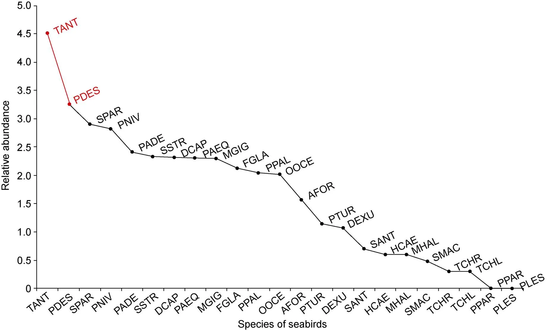
Figure 1 Rank abundance curve shows relative species abundance (log scale) in the whole study area. Species in red represent more than 90% of the total abundance obtained throughout the study. Species names as in Table 1.

Table 1 Total numbers of seabirds registered between December 2019 and January 2020. The four-letter codes following the scientific names of the birds identify the species in Figure 2

The distribution model was applied to the most abundant species, Antarctic petrel. Receiver operating characteristic curve (ROC) is a widely used model evaluation index. The area value surrounded by the coordinate axis under the ROC curve is the AUC (area under the curve) value, which is used as the standard to judge the quality of the model (Wang et al., 2007). The AUC value of the Antarctic petrel species distribution model simulated by Maxent is 0.802, which is greater than 0.8, indicating that the model prediction is not random and the prediction result is reliable. The potential habitat of Antarctic petrel is mainly located in the region near the ocean front, and the northern sea area of Lützow-Holm Bay (30°E–40°E) is the most concentrated (Figure 3).

Environmental factors generally contributing more than 60% in the model construction are considered to have a major impact on the distribution of Antarctic petrel. The contribution rate of variables from large to small is: sea ice thickness 52.5%, current velocity 30.4% and sea water salinity 17.1%. Sea ice thickness accounting for more than half of the model contribution, but none of the three variables could be considered as the major effect factors. Sea ice thickness has the most useful information by itself, but salinity was the main information that isn’t present in the other variables.

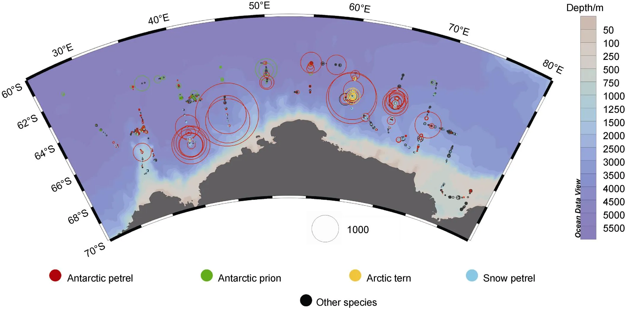
Figure 2 Distributions and group sizes of seabirds in the Cosmonaut Sea and surrounding areas between December 2019 and January 2020. The circle size represents the observed group size. The circle color indicates different species.

Figure 3 Potential suitable habitat of Antarctic petrel. Warmer colors show areas with better predicted conditions. The value represents the spatial distribution probability of Antarctic petrel.

4 Discussion

Our study provides a picture of the status of seabirds in the Cosmonaut Sea and the surrounding area in Antarctica. Previous records on seabirds have come from surveys conducted mostly to study marine science since the early 1970s (Khimitsa, 1976). These surveys have been temporally spaced over a period of 15 years and thus the existing information on seabird distribution in these areas has mostly been patchy or anecdotal in origin (Woehler et al., 2010). With at least 23 different species, species diversity observed during this study was slightly higher than the previous studies in the Cosmonaut Sea (Woehler et al., 2010). In comparison to other studies both in adjacent sectors of the Antarctic like Prydz Bay (Woehler et al., 2003), and elsewhere in the Southern Ocean (Joiris, 1991; Pande et al., 2020), the composition of species is similar. It is clear that the ice-associated seabird assemblage is ubiquitous in the Southern Ocean close to the Antarctic continent.

Few species exhibited high abundances. Antarctic petrel (about 32700) and Antarctic prion (about 1800) had observed more than 1000 individuals, followed by Arctic tern () (about 800) and Snow petrel () (about 650). The number of other species recorded was less than 300 individuals. ​The connection between high concentrations and low species diversity seems to reflect both high biological productivity and low biodiversity in the Sub-Antarctic and Polar Fronts (Joiris and Humphries, 2018). Nearly half of seabird species (11 of 23) had sights less than 50 individuals. This scenario is typical in Antarctic marine ecosystem and was already described decades ago (Watson, 1975). As is common in other oceans, hotspots of high bird abundance and richness occurred in the presence of highly productive coastal or marine fronts. Many of our observations (Figure 4) were obtained at the South of the front of the ACC, which has been described as a critical component of the global ocean circulation (Orsi et al., 1995) that provides predictable productive foraging for many species (Tynan, 1998). There are also some hotspots (Figure 4) at the confluence of fast currents.

There were notable differences in species diversity and abundance between different latitude zones. Abiotic and biotic oceanographic processes and their interactions influence the distribution and abundance of seabirds at sea in the Southern Ocean (e.g., Woehler et al., 2010). The open-water community usually exhibits greater diversity and variability in its composition (Woehler, 1997; Woehler et al., 2003, 2006). In this study, the zone close to high sea recorded more bird species than near continental shelf. The zone near the continental shelf has the smallest ocean area, explaining part of the low abundances and richness. Although some penguins can disperse on distances traversing major Southern Ocean fronts (Thiebot et al., 2011, 2012), most are natally philopatric (Seddon et al., 2013), no records in high sea region is within the expected distribution pattern for this species.

Figure 4 Seabirds hotspots and the major circulation features of the Cosmonaut Sea. Including the eastward flowing Coastal Current (CC), the Antarctic Circumpolar Current (ACC) and its Southern Boundary (SB) (Orsi et al., 1995).

Most areas with better predicted conditions congregate in the region near ocean front, where also shows the best species abundance and richness in our investigation. Different flow with eddy current, upwelling and other characteristics and the subsequent hydrodynamic processes have the potential to generate different small-scale oceanographic features, which could gather a large number of phytoplankton and fish (Holm and Burger, 2002). The important upwelling and ACC in the Southern Ocean not only provide a lot of resources for foraging seabirds, but also provide clues for us to predict the aggregation area of seabirds. Among the variables in the model, the thickness of sea ice, which comprehensively displays the distribution of pack ice and icebergs, has the greatest impact on the distribution of Antarctic petrel. It may be because more fish and krill gather on the edge of sea ice than in the open sea, which could influence the availability of profitable foraging resources for seabirds (Haberman et al., 2003).

There are still some limitations in this survey. Variability amongst different observers is a potential source of data variability due to inter-observer biases (Ryan and Cooper, 1989). Another potential source of error is the presence of the vessel influencing the behaviour at sea of the seabirds observed (Woehler et al., 2003). Some species are known to be attracted to vessels, such as albatrosses, skuas and fulmarine petrels (Ryan and Cooper, 1989; Woehler, 1997). The low frequency of sightings for some species (e.g., Parkinson’s petrel) may reflect their scarcity in the survey area or their behavioural preferences in regard to being attracted to, or avoiding vessels. Also, the phenomenon of large aggregations indicated if some hotspots were undetected, collected observations would lead to an underestimation of the actual numbers and a wrong prediction of the distribution (Joiris, 2011, 2018; Joiris and Humphries, 2018). We only selected one dominant species to build the species distribution model, but different species may have different distribution patterns due to their diet and reproductive behaviors. Also, we use three environmental variables to predict and simulate the potential distribution area of species. In fact, the actual distribution area of species is also affected by many factors, for example, the physiological tolerance of species to climate change (Sun et al., 2000) and the impact of human activities (Yogui and Sericano, 2009).

We are grateful to all the members of the 36th CHINARE. This study was financially supported by National Polar Special Program “Impact and Response of Antarctic Seas to Climate Change” (Grant nos. IRASCC2020-2022-05, IRASCC2020-2022-06). Finally, the authors would like to acknowledge the reviewer, Dr. Claude R. Joiris for his valuable comments, which greatly helped improve this paper.

This paper is a solicited manuscript of Special Issue “Marine Ecosystem and Climate Change in the Southern Ocean” published on Vol.33, No.1 in March 2022.

Barbraud C, Delord K C, Micol T, et al. 1999. First census of breeding seabirds between Cap Bienvenue (Terre Adélie) and Moyes Islands (King George V Land), Antarctica: new records for Antarctic seabird populations. Polar Biol, 21(3): 146-150, doi:10.1007/s003000050345.

Barth J A, Cowles T J, Pierce S D. 2001. Mesoscale physical and bio-optical structure of the Antarctic Polar Front near 170°W during austral spring. J Geophys Res, 106(C7): 13879-13902, doi:10.1029/ 1999jc000194.

Becker E, Forney K, Fiedler P, et al. 2016. Moving towards dynamic ocean management: how well do modeled ocean products predict species distributions? Remote Sens, 8(2): 149, doi:10.3390/rs8020149.

Bibik V A, Maslennikov V V, Pelevin A S, et al., 1988. The current system and the distribution of waters of different modifications in the Cosmonaut Sea//Lubimova T G, Makarov R R, Maslennikov V V, et al. Interdisciplinary investigations of pelagic ecosystem in the Commonwealth and Cosmonaut Seas. Moscow: VNIRO Publishers, 16-43.

Bundichenko E V, Khromov N S, 1988. Mesoplankton biomass, age composition and distribution of dominant species in relation to water structure in the Commonwealth and the Cosmonaut Seas//Lubimova T G, Makarov R R, Maslennikov V V, et al. Interdisciplinary investigations of pelagic ecosystem in the Commonwealth and Cosmonaut Seas. Moscow: VNIRO Publishers, 83-109.

Cimino M A, Fraser W R, Irwin A J, et al. 2013. Satellite data identify decadal trends in the quality of Pygoscelis penguin chick-rearing habitat. Glob Chang Biol, 19(1): 136-148, doi:10.1111/gcb.12016.

Clarke E D, Spear L B, McCracken M L, et al. 2003. Validating the use of generalized additive models and at-sea surveys to estimate size and temporal trends of seabird populations. J Appl Ecol, 40(2): 278-292, doi:10.1046/j.1365-2664.2003.00802.x.

Davidson A T, Scott F J, Nash G V, et al. 2010. Physical and biological control of protistan community composition, distribution and abundance in the seasonal ice zone of the Southern Ocean between 30 and 80°E. Deep Sea Res Part II Top Stud Oceanogr, 57(9-10): 828-848, doi:10.1016/j.dsr2.2009.02.011.

Elith J, Leathwick J R. 2009. Species distribution models: ecological explanation and prediction across space and time. Annu Rev Ecol Evol Syst, 40: 677-697, doi:10.1146/annurev.ecolsys.110308.120159.

Elith J, Phillips S J, Hastie T, et al. 2011. A statistical explanation of MaxEnt for ecologists. Divers Distrib, 17(1): 43-57, doi:10.1111/j. 1472-4642.2010.00725.x.

Franklin J. 2009. Mapping species distributions: spatial inference and prediction. Cambridge: Cambridge University Press, 1-320.

Frederiksen M, Edwards M, Richardson A J, et al. 2006. From plankton to top predators: bottom-up control of a marine food web across four trophic levels. J Anim Ecol, 75(6): 1259-1268, doi:10.1111/j.1365- 2656.2006.01148.x.

Guisan A, Tingley R, Baumgartner J B, et al. 2013. Predicting species distributions for conservation decisions. Ecol Lett, 16(12): 1424-1435, doi:10.1111/ele.12189.

Haberman K L, Ross R M, Quetin L B. 2003. Diet of the Antarctic krill (): II. Selective grazing in mixed phytoplankton assemblages. J Exp Mar Biol Ecol, 283(1-2): 97-113, doi:10.1016/S0022-0981(02)00467-7.

Holm K J, Burger A E. 2002. Foraging behavior and resource partitioning by diving birds during winter in areas of strong tidal currents. Waterbirds, 25(3): 312-325, doi:10.1675/1524-4695(2002)025[0312: fbarpb]2.0.co;2.

Joiris C R. 1991. Spring distribution and ecological role of seabirds and marine mammals in the Weddell Sea, Antarctica. Polar Biol, 11(7): 415-424, doi:10.1007/BF00233076.

Joiris C R. 2011. A major feeding ground for cetaceans and seabirds in the south-western Greenland Sea. Polar Biol, 34(10): 1597-1607, doi:10.1007/s00300-011-1022-1.

Joiris C R. 2018. Seabird and marine mammal “hotspots” in polar seas. Lambert: Düsseldorf.

Joiris C R, Humphries G R W. 2018. Hotspots of seabirds and marine mammals between New Zealand and the Ross Gyre: importance of hydrographic features. Adv Polar Sci, 29(4): 254-261, doi: 10.13679/j. advps.2018.4.00254.

Kaschner K, Quick N J, Jewell R, et al. 2012. Global coverage of cetacean line-transect surveys: status quo, data gaps and future challenges. PLoS One, 7(9): e44075, doi:10.1371/journal.pone.0044075.

Khimitsa V A. 1976. Investigation of geostrophic currents in the Antarctic zone of the Indian Ocean. Oceanology, 16(2), 131-133.

Kochergin A T, Mikhailovsky Y A, Mikhal’tseva T V. 1988. Hydro- chemical conditions of biological productivity formation in the Cosmonaut and Commonwealth Seas//Lubimova T G, Makarov R R, Maslennikov V V, et al. Interdisciplinary investigations of pelagic ecosystem in the Commonwealth and Cosmonaut Seas. Moscow: VNIRO Publishers, 63-69.

Lascelles B G, Langham G M, Ronconi R A, et al. 2012. From hotspots to site protection: identifying Marine Protected Areas for seabirds around the globe. Biol Conserv, 156: 5-14, doi:10.1016/j.biocon.2011.12.008.

Makarov R R, Savich M S, 1988. Peculiarities of the distribution and biomass of phytoplankton in the Cosmonaut and Commonwealth Seas in January–February 1984//Lubimova T G, Makarov R R, Maslennikov V V, et al. Interdisciplinary Investigations of Pelagic Ecosystem in the Commonwealth and Cosmonaut Seas. Moscow: VNIRO Publishers, 69-83.

Marshall C E, Glegg G A, Howell K L. 2014. Species distribution modelling to support marine conservation planning: the next steps. Mar Policy, 45: 330-332, doi:10.1016/j.marpol.2013.09.003.

Moore J K, Abbott M R. 2002. Surface chlorophyll concentrations in relation to the Antarctic Polar Front: seasonal and spatial patterns from satellite observations. J Mar Syst, 37(1-3): 69-86, doi:10.1016/S0924- 7963(02)00196-3.

Orgeira J L. 2018. Occurrence of seabirds and marine mammals in the pelagic zone of the Patagonian Sea and north of the South Orkney Islands. Adv Polar Sci, 29(1): 25-33, doi: 10.13679/j.advps.2018.1. 00025.

Orgeira J L, Alderete M C, Jiménez Y G, et al. 2015. Long-term study of at-sea distribution of seabirds and marine mammals in the Scotia Sea, Antarctica. Adv Polar Sci, 26(2): 158-167, doi: 10.13679/j.advps.2015. 2.00158.

Orsi A H, Whitworth T III, Nowlin. W D. 1995. On the meridional extent and fronts of the Antarctic Circumpolar Current. Deep Sea Res Part I Oceanogr Res Pap, 42(5): 641-673, doi:10.1016/0967- 0637(95) 00021-W.

Paleczny M, Hammill E, Karpouzi V, et al. 2015. Population trend of the world’s monitored seabirds, 1950–2010. PLoS One, 10(6): e0129342, doi:10.1371/journal.pone.0129342.

Pande A, Mondol S, Sathyakumar S, et al. 2020. Past records and current distribution of seabirds at Larsemann Hills and Schirmacher Oasis, east Antarctica. Polar Rec, 56: e40, doi:10.1017/s0032247420000364.

Phillips S J, Anderson R P, Schapire R E. 2006. Maximum entropy modeling of species geographic distributions. Ecol Model, 190(3-4): 231-259, doi:10.1016/j.ecolmodel.2005.03.026.

Robinson L M, Elith J, Hobday A J, et al. 2011. Pushing the limits in marine species distribution modelling: lessons from the land present challenges and opportunities. Glob Ecol Biogeogr, 20(6): 789-802, doi:10.1111/j.1466-8238.2010.00636.x.

Ryan P G, Cooper J. 1989. Observer precision and bird conspicuousness during counts of birds at sea. S Afr J Mar Sci, 8(1): 271-276, doi:10.2989/02577618909504567.

Sarmiento J L, Hughes T M C, Stouffer R J, et al. 1998. Simulated response of the ocean carbon cycle to anthropogenic climate warming. Nature, 393(6682): 245-249, doi:10.1038/30455.

Sarmiento J L, Le Quéré C. 1996. Oceanic carbon dioxide uptake in a model of century-scale global warming. Science, 274(5291): 1346-1350, doi:10.1126/science.274.5291.1346.

Schwarz J N, Raymond B, Williams G D, et al. 2010. Biophysical coupling in remotely-sensed wind stress, sea surface temperature, sea ice and chlorophyll concentrations in the South Indian Ocean. Deep Sea Res Part II Top Stud Oceanogr, 57(9-10): 701-722, doi:10.1016/j. dsr2.2009.06.014.

Seddon P J, Ellenberg U, Heezik Y V. 2013. Yellow-eyed penguin. Washington: University of Washington Press.

Sun L, Xie Z, Zhao J. 2000. A 3,000-year record of penguin populations. Nature, 407(6806): 858, doi:10.1038/35038163.

Thiebot J B, Cherel Y, Trathan P N, et al. 2011. Inter-population segregation in the wintering areas of macaroni penguins. Mar Ecol Prog Ser, 421: 279-290, doi:10.3354/meps08907.

Thiebot J B, Cherel Y, Trathan P N, et al. 2012. Coexistence of oceanic predators on wintering areas explained by population-scale foraging segregation in space or time. Ecology, 93(1): 122-130, doi:10. 1890/11-0385.1.

Thomson P G, Davidson A T, van den Enden R, et al. 2010. Distribution and abundance of marine microbes in the Southern Ocean between 30 and 80°E. Deep Sea Res Part II Top Stud Oceanogr, 57(9-10): 815-827, doi:10.1016/j.dsr2.2008.10.040.

Tynan C T. 1998. Ecological importance of the Southern Boundary of the Antarctic Circumpolar Current. Nature, 392(6677): 708-710, doi:10.1038/33675.

Wang Y S, Xie B Y, Wan F H, et al. 2007. Application of ROC curve analysis in evaluating the performance of alien species’ potential distribution models. Biodivers Sci, 15(4): 365-372 (in Chinese with English abstract).

Watson G. 1975. Birds of the Antarctic and Sub-Antarctic. Washington: American Geophysical Union.

Westwood K J, Brian Griffiths F, Meiners K M, et al. 2010. Primary productivity off the Antarctic coast from 30°–80°E; BROKE-West survey, 2006. Deep Sea Res Part II Top Stud Oceanogr, 57(9-10): 794-814, doi:10.1016/j.dsr2.2008.08.020.

Wiley E O, McNyset K, Peterson T, et al. 2003. Niche modeling perspective on geographic range predictions in the marine environment using a machine-learning algorithm. Oceanography, 16(3): 120-127, doi:10.5670/oceanog.2003.42.

Woehler E J. 1997. Seabird abundance, biomass and prey consumption within Prydz Bay, Antarctica, 1980/1981–1992/1993. Polar Biol, 17(4): 371-383, doi:10.1007/PL00013379.

Woehler E J, Raymond B, Boyle A, et al. 2010. Seabird assemblages observed during the BROKE-West survey of the Antarctic coastline (30°E–80°E), January–March 2006. Deep Sea Res Part II Top Stud Oceanogr, 57(9-10): 982-991, doi:10.1016/j.dsr2.2008.12.041.

Woehler E J, Raymond B, Watts D J. 2003. Decadal-scale seabird assemblages in Prydz Bay, East Antarctica. Mar Ecol Prog Ser, 251: 299-310, doi:10.3354/meps251299.

Woehler E J, Raymond B, Watts D J. 2006. Convergence or divergence: where do short-tailed shearwaters forage in the Southern Ocean? Mar Ecol Prog Ser, 324: 261-270, doi:10.3354/meps324261.

Yogui G T, Sericano J L. 2009. Levels and pattern of polybrominated diphenyl ethers in eggs of Antarctic seabirds: endemic versus migratory species. Environ Pollut, 157(3): 975-980, doi:10.1016/j. envpol.2008.10.016.

10.13679/j.advps.2021.0028

30 September 2021;

5 September 2022;

30 September 2022

: Lin Z X, Liu M J, Yan D H, et al. Population size and distribution of seabirds in the Cosmonaut Sea, Southern Ocean. Adv Polar Sci, 2022, 33(3): 291-298,doi:10.13679/j.advps.2021.0028

, ORCID: 0000-0002-2355-567x, E-mail: dengwh@bnu.edu.cn