Environmental heterogeneity regulates species-area relationships through the spatial distribution of species

Chenqi He, Leqi Fng, Xinyu Xiong, Fn Fn, Yngng Li, Luoshu He, Xioli Shen,Sheng Li, Chengjun Ji, Jingling Zhu,＊

a Institute of Ecology, College of Urban and Environmental Sciences, Key Laboratory for Earth Surface Processes of the Ministry of Education, Peking University, Beijing,100871, China

b School of Life Sciences, Peking University, Beijing, 100871, China

c State Key Laboratory of Vegetation and Environmental Change, Institute of Botany, Chinese Academy of Sciences, Beijing, 100093, China

Keywords:Plants life forms Species-area curves Sampling design Spatial pattern Species diversity

ABSTRACT Species-area relationships (SARs), also known as species-area curves, are fundamental scaling tools for biodiversity research. Sampling design and taxonomic groups affect the widely cited forms of species-area curves.However, the influence of sampling design and related environmental heterogeneity on SAR curves is rarely considered.Here,we investigated the SAR among different plant life forms(herbaceous plants,shrubs,and trees)in a 25.2-ha ForestGEO plot,the Wanglang Plot,in Sichuan,southwestern China,using a non-contiguous quadrat sampling method and power-law model.We compared the estimated parameters(the intercept c and the slope z)of the power-law models among different plant life forms, tested whether the SAR curve forms varied with sampling starting location, and assessed the effect of environmental heterogeneity accumulating with sampling area on curve variation.We found a wider range of variations in the SARs.The estimated c,z-values of power SAR were higher for the herbaceous plants than for the woody plants. A wider variation of SARs for the herbaceous plants than those for the woody plants. The selection of sampling starting location affected the SAR curve forms because of the roles of soil and topographic heterogeneity. We concluded that environmental heterogeneity regulates SAR curves sampled from different starting locations through spatial distribution of plant life forms.Thus, we recommend considering the design of sampling starting location when constructing SAR curves, especially in a heterogeneous habitat with unrandom distribution patterns of species.

1. Introduction

Species-area relationship (SAR) describes an increase in species number with sampling area, representing one of the most fundamental laws of ecology (Lomolino, 2000). As an effective tool for interpolation and extrapolation of biodiversity across different scales, species-area relationship and corresponding mathematical models have been widely applied to the equilibrium theory of island biogeography, biodiversity hotspot identification, and nature reserve design (Losos and Schluter,2000;Guilhaumon et al.,2008;Rybicki and Hanski,2013;Meixler et al.,2019;Schrader et al.,2020).Various feasible mathematical models have been employed to describe SARs,among which the power function(also called the power law)is the most commonly used model for biologically meaningful parameter estimation(Sizling and Storch,2004;Martin and Goldenfeld,2006).

The formats and parameters of the SARs depend largely on the sampling design (for example, the starting location of the nested plots),especially in heterogeneous habitats, such as in mountainous areas(Drakare et al.,2006;Beck and Kitching,2009;Bueno et al.,2020).For instance, a nest-sampling or random-sampling design with coarse series sampling quadrats may obscure diversity variation resulting from the spatial distribution pattern of species in heterogeneous habitats (Ulrich and Buszko,2007;Reinhard and Drossel,2021).Many researchers have found the influences of sampling design on the SAR, such as nested or independent sampling, scale and grain size of the design, and sampling intensity, influence the diversity-scale relationships when utilizing SAR tools to estimate species diversity patterns of plant communities(McGlinn and Palmer, 2009; Azovsky, 2011). Sampling design with varying starting locations and corresponding directions may illustrate different SAR curves and how species diversity changes with the area.For example,in a 50-ha plot,He et al.(1996)found that the sampling starting location significantly affected the SAR formats because of the spatial heterogeneity.However,previous studies have widely based on random selection or from the corner of a plot as the starting location of the sampling design (Scheiner, 2003). The influences of sampling starting location on the SARs and the spatial diversity pattern have often been ignored(Shmida,1984).In this sense,it is critical to evaluate how SARs varied with sampling design, especially the sampling starting location before the SARs can be applied to extrapolate or interpolate species richness.

Environmental heterogeneity is a prevalent factor regulating species richness patterns(Scheiner et al.,2011;Stein et al.,2014;Schrader et al.,2020),it may also affect the formats and parameters of SARs.The efficacy of SAR varies with within-fragment heterogeneity(Giladi and Ziv,2020).The environmental variables might explain high variance in the slope of SAR curves under nested sampling along an environmental heterogeneity gradient (Desilets and Houle, 2005). Many previous studies have illustrated the influence of species spatial distribution and abundance distribution on SARs, and that uneven occupancies and aggregation may result in steeper SARs(He and Legendre,2002;Tjørve et al.,2008;Qiao et al., 2012; DeMalach et al., 2019). Environmental heterogeneity may affect SARs indirectly through the spatial distribution and abundance distribution of species (He and Legendre, 2002). Species spatial distribution is a bridge to construct SAR curves in connection with sampling design and environmental heterogeneity(He and Legendre,2002;Tjørve et al., 2008). Sampling design from different starting locations reveals SARs change with species diversity at origins and spatial distribution patterns. How environmental heterogeneity affects SAR formats from different sampling starting locations answers whether the environment regulates SARs through spatial distribution of species. What's more, the mechanism by which environmental heterogeneity influences SAR formats between plant life forms in the Wanglang Plot remains unclear.

It is widely acknowledged that models of SARs differ among taxonomic groups and habitats(Drakare et al.,2006),possibly because of the dispersal ability differences between species and individual organisms(Shen et al.,2009).The distant spreader,such as the herbaceous plants,may result in flatter SAR because of their higher dispersal abilities,than those with short disperse distances,such as woody plants(Drakare et al.,2006). Even within the same taxonomic group and habitat type, some studies have observed different patterns of SAR (Keeley and Fotheringham, 2003; Page et al., 2010). For example, California shrublands are dominated by Mediterranean-type plant communities, but the slope of the SAR curves of herbaceous and woody plants was inconsistent with other Mediterranean-type shrublands(Keeley and Fotheringham,2003).

In this study,we investigated how SARs change with plant life forms and sampling starting location, and how environmental heterogeneity contributes to the variation of SARs in a subalpine coniferous forest dynamics plot,the Wanglang Plot,in Sichuan,southwestern China,aiming to answer the following questions.

First,how do SARs differ between plant life forms?We hypothesized a steeper SAR curve (larger slope in a logarithm-transformed space) for woody plants than that for herbaceous plants,and a steeper one for trees than shrubs, because the larger sized organisms, i.e., woody plants,dispersed more limitedly (and therefore less homogeneous) than the smaller sized ones,i.e.,herbaceous plants(Drakare et al.,2006).

Second, how does sampling starting location affect SARs? We hypothesized lower slopes of SARs for plot series starting at homogeneous localities than those starting at heterogeneous localities because homogeneous localities tended to increase the species distribution homogenization,which decreased the species turnover and lowered the slopes of the SARs(He and Legendre,2002;Tjørve et al.,2008).

Third,how do environmental factors influence SAR variations under a specific spatial distribution pattern? We hypothesized that SARs from different starting sampling locations varied more remarkably for the woody plants than for the herbaceous plants. We had this hypothesis because environmental heterogeneity partly shaped the spatial distribution of plant life forms (He and Legendre, 2002; Stein et al.,2014). Herbaceous plants dispersed further and adapted to a wider environmental range, leading to higher homogenization of species compositions (Hovestadt and Poethke, 2005), than woody plants. In contrast, woody plants had dispersal limitations and deterministic processes shaping their local species richness more heterogeneous, especially in non-tropical forests (Wang et al., 2016, 2018). We further hypothesized that higher variance was explained by environmental heterogeneity in the variances of SARs for woody plants, indicating a heterogeneous environment that varied construction of SARs through species spatial distribution patterns than herbaceous plants.

2. Materials and methods

2.1. Study site

The 25.2-ha Wanglang Plot is located in Wanglang National Nature Reserve(103°55′–104°10′E,32°49′–33°02′N;Fig.1),Sichuan Province of China, which is located in the core habitat of the giant panda in the north of Minshan Mountain,at an altitude range of 2,850–2,930 m.The climate is humid monsoon,with a mean annual precipitation of ca.866.5 mm and a mean annual temperature of 2.9°C.The main vegetation type in the reserve is subalpine dark coniferous forest, dominated by Abies faxoniana and Picea purpurea in the tree layer and Philadelphus purpurascens and Sorbus koehneana in the shrub layer.

2.2. Vegetation survey

The 25.2-ha(360 m×700 m)Wanglang Plot consists of 630 quadrats(18 rows and 35 columns), each with an area of 20 m × 20 m. We investigated the woody plants in the plot according to the Centre for Tropical Forest Science(CTFS).Specifically,we located and identified all living woody plant species with a diameter of 1 cm. Based on plant life forms,we classified woody plants into two categories,tree and shrub(Wu et al., 1994). In addition, we investigated the herbaceous layer in 212 quadrats distributed evenly in the plot, identifying and recording the species names of all existing herbaceous plants in each quadrat.In total,we recorded 274 plant species,including 230 herbaceous,25 shrub,and 19 tree species.

2.3. Construction of SARs

We constructed SARs for shrub, tree and herbaceous species for the nested samples originated from each quadrat (Fig. 1a and b). We fitted the SAR data with the log-transformed power model (Eq. (1)) for the three plant life forms

where S is species richness,A is the sampling area(number of quadrats),and c and z are the estimated parameters.The c-value is species richness per unit area, and the z-value is often viewed as a measure of beta diversity(Crist and Veech,2006;Tjørve and Tjørve,2008).A species-area curve with higher c and lower z-values represented relatively high alpha diversity around the sampling starting location and low species composition variation (Crist and Veech, 2006; Chase et al., 2018), which indicates a more homogeneous species spatial distribution pattern. In contrast,lower c and higher z-values indicate a more aggregative spatial distribution pattern(DeMalach et al.,2019).

Fig.1. Geographical location(a)of the subalpine coniferous forest dynamics plot(the Wanglang Plot)in Sichuan,China,with a remote sensing image displaying the vegetation coverage of the site(b).Schematic diagram of the sampling design to construct a species-area relationship(SAR)(c).The grey cells represent the quadrats,and the red one represents sampling starting location.The sampling rule is clockwise.(For interpretation of the references to colour in this figure legend,the reader is referred to the Web version of this article.)

Specifically, we first counted the number of species in each quadrat and then expanded the sampling area with a clockwise rule and counted the total number of species (Fig. 1c). For a relatively small area, the numbers of adjacent quadrats were added according to the geometric law of 1, 2, 4, 8, 16, and then 10 adjacent quadrats were added every time according to the arithmetic law. As a result, we obtained the sampling areas of 1,2,4,8,16,26,36,46,…,212.To gain the same sampling area levels between different plant life forms for comparison,we constructed SARs of the herbaceous and woody species with 212 quadrats respectively.In fact,the expansion of the sampling area for Type III curves was represented by the addition of quadrats (Scheiner, 2003). We summarised species richness at each level of the combined quadrats and obtained a relationship between species richness and quadrat quantity.Finally,we obtained 212 species-area curves for trees, shrubs, and herbaceous plants.

2.4. Environmental heterogeneity

The environmental heterogeneity of a forest dynamics plot is mainly manifested in changes in soil physicochemical properties and spatial topography, which determines the pattern of plant diversity aboveground(Bin et al.,2010;Xue et al.,2019;Heidrich et al.,2020).Five soil samples were taken at the midpoint and four corners within a 20 m×20 m quadrat.We sampled soil of 98 quadrats distributed evenly in the plot.To eliminate the collinearity of multiple environmental factors, we selected nine empirical and representative environmental factors affecting the distribution of species diversity: the slope, aspect, altitude(m), soil bulk density (g⋅m-3), soil total carbon content (kg⋅m-2), soil total nitrogen content (kg⋅m-2), soil pH, soil temperature (°C) and soil moisture (%). The spatial distribution of environmental factors was obtained with Ordinary Kriging interpolation, which is commonly applied in other biodiversity research (Fortin and Dale, 2005; Kreft and Jetz,2007). We used an exponential variogram model and optimized the number of lags and lag size, and then test the model availability according to RMS(Root Mean Square)and standardised RMS.The Kriging spatial interpolation was analyzed in the Geostatistical Analyst Module of ArcGIS 10.3(Fortin and Dale, 2005).

Subsequently, all variables were standardised to a mean of 0 and a standard deviation of 1 for further analysis. We calculated the standard deviation of the specific environmental factor(Eij)at the ithsampling area level (Ai, i in 1, 2, 3, …, m, where m is the maximum sampling area) to indicate environmental heterogeneity from the jthsampling starting location(j in 1,2,3,…,n,where n is the maximum number of sampling starting locations). Accordingly, the standard deviation of the environmental factor(E1j)was zero for the first sampling area level(A1),and the environmental heterogeneities of the second(A2)and third(A3)sampling area levels were E2jand E3j,respectively.With increasing sampling area and species richness,the environmental heterogeneity gradient(E1j,E2j,E3j,…,Eii,…,Emj)within each sampling area level(A1,A2,A3,…,Ai,…,Am) corresponded to the jthspecies-area curve. All species-area curves from a different starting location had an environmental heterogeneity gradient associated with the sampling area and mainly depended on their local environmental conditions.

2.5. Statistical analyses

We used a sampling approach based on computer simulation and fitted species-area models with a log-transformed power model SAR(Eq.(1))for the three plant life forms.We further defined a mismatch of the jthspecies-area curves at the ithsampling area level with the mean species richness-area relationship by a variation coefficient δij(Fig.2,Eq.(2)):

where Airepresents the sampling area level.The f（c0，z0，A）is the mean species richness-area relationship,as we also calculated the mean species richness at each level of the sampling area.We regarded the f（c0，z0，A）as the general SAR of the Wanglang plot and compared it with other SARs constructed by different sampling starting locations.The f（cj，zj，A）was a SAR function built at the jthsampling starting location. When the f（cj，zj，A）curve was entirely higher or lower than the general SAR f（c0，z0，A）,δijwas always positive or negative(Fig.2).However,when two curve functions existed at an intersection,some integral regions were positive,some were negative,and the entire variation coefficient δmjtoward 0.We compared all sampling origination-based species-area curves with the general SAR and calculated δijfor each curve(j)and sampling area level(i).

To evaluate the bias of model fitting on the variation of SARs,we also calculated the variation coefficient δijusing empirical SARs without fitting SAR models.We defined the δijas a mismatch between the species richness at each level of the sampling area(Eq.(3)):

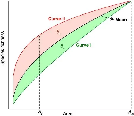
Fig. 2. Diagram of defining the variation coefficient δij for species-area curves.The black curve f（c0，z0，A） represents the mean species richness-area relationships(the general SAR)in the plot.Curve I and II represents the jth speciesarea relationships f（cj，zj，A） with relatively lower and higher species richness around sampling starting locations, respectively. The variation coefficient δij of the jth species-area curves is the portion of the shadow area below the limit of Ai.The entire variation δmj of curves f（cj，zj，A）based on the general SAR in the plot was indicated by the shadow area below the limit of the maximum sampling area Am (Red: positive variations δ+; Green: negative δ–). (For interpretation of the references to colour in this figure legend, the reader is referred to the Web version of this article.)

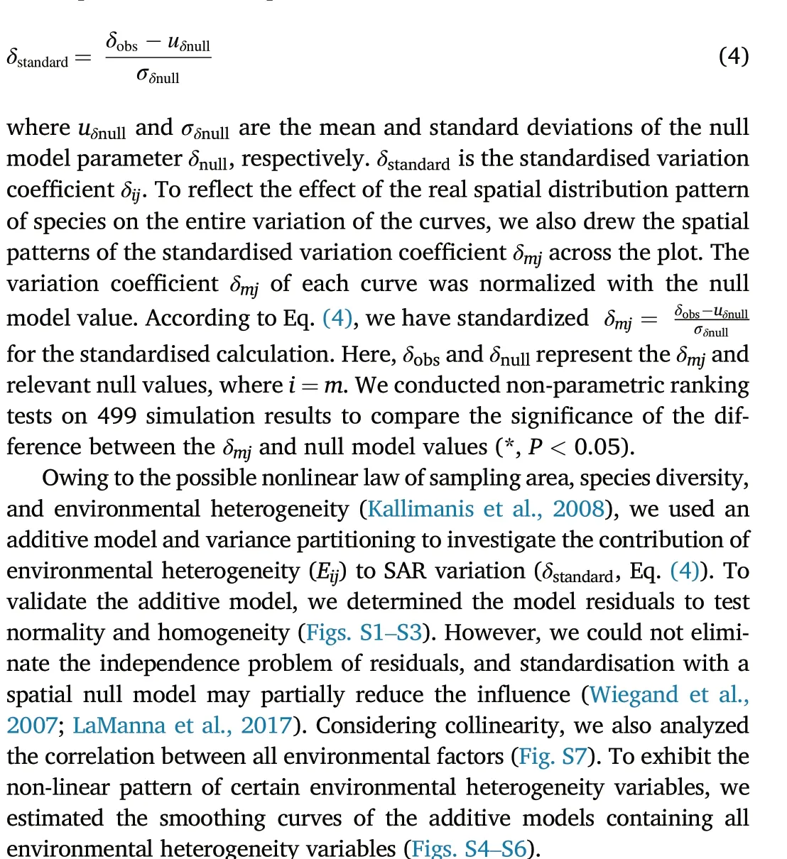
To depict the species spatial distribution effect contributing to SAR variation and to exclude the interference of stochasticity,we simulated a completely random distribution null model based on the species occupancy of a plot(species occupancy=real species occurrence/maximum quadrat number)(Tjørve et al.,2008;Qiao et al.,2012).Each species had the same probability of being located in any quadrat, but the sum of species occurrence relied on the real species occurrence. If a species occurred in a quadrat,the real species occurrence increased by one.After inspecting all quadrats, the real species occurrence was the overall species occurrence in the plot. We ran 499 Monte Carlo simulations to generate species random distribution and SAR under the null model,then fitted the null SAR with a log-transformed power model (Eq. (1)). We calculated the corresponding variation coefficient δijusing Eqs. (2) and(3). Non-parametric ranking tests were performed to evaluate the significant differences between the real parameter values and null values(α= 0.05). The null model was also used for standardisation to assess the effect of species spatial distribution patterns on SAR variation. We standardised the real variation coefficient δij(δobs)with the relevant null model parameter δnull(Eq.(4)):

We classified environmental factors into two groups: soil heterogeneity, which included heterogeneity in soil total carbon content, total nitrogen content, pH, moisture, and bulk density, and topographic heterogeneity, which included heterogeneity in slope, aspect, and altitude.We compared the explained deviances (R2) of the two groups and their interactions with the SAR. To estimate the relative effects of environmental factors, we calculated the explained deviances of the single predictor(the“single-term”models)and evaluated their performance using the full models(Table S1).

The R package ‘mgcv’ was used for model analysis and fitting (Zuur et al.,2009).Variables and optimal models were evaluated and selected through p-values, generalized cross validation (GCV), and Akaike information criterion (AIC). All calculations were performed in R 4.0.5 (R Core Team,2020).

3. Result

3.1. Characteristics of the SAR among life forms

In general, the estimated parameters of the power-law SAR varied among plant life forms (Fig. 3). SARs of the herbaceous plants had the highest c-values(46.55),followed by those of the shrubs(11.42)and the trees(5.96)(Fig.3),indicating higher mean species richness around the quadrats for the herbaceous plants than for the woody plants. The zvalues of the power model were lower in the shrubs (0.16) and trees(0.20) than in herbaceous plants (0.32) (Fig. 3), indicating that species spatial distribution is largely dependent on plant life forms.

3.2. Changes in SARs with the sampling starting location

The pattern of standardised δmjrevealed that the SARs varied remarkably among different samples (Fig. 4a–c). The fitting bias of the power model had little effect on the variation(Fig.S8).After eliminating the effects of stochasticity with the null model, the forms of some SARs constructed from various sampling starting locations were still different from the general SAR(the mean species-area curves of the plot).For the herbaceous plants,84%of the SARs were different from the general SAR.These proportions were 19% and 2% for the shrubs and the trees,respectively.Moreover,the spatial patterns of the standardised δmjwere opposite in the upper and lower regions of the plot for the herbaceous plants,suggesting that the SARs sampled starting from the upper regions occupied higher local species richness than the general SAR.In contrast,the curves from the lower regions were integrally lower than the general SAR. The patterns of the standardised δmjfor the woody plants were spatially different from those of the herbaceous plants,indicating that the plant life forms influenced the variation of SARs with sampling starting locations. The SARs of the herbaceous plants contained a larger standardised δmjthan those of the woody plants (Fig. 4d), which further indicated a more spatially aggregative and more heterogeneous distribution for the herbaceous than the woody plants.

3.3. Effects of environments on the SAR

The additive model reflected the non-linear relationships between environmental heterogeneity and the standardised δmj(Figs. S4–S6). The variance partitioning showed that topographic and soil heterogeneities contributed significantly to the variance in SARs, explaining more variation in the standardised δmjin the herbaceous plants(52.70%)than in the shrubs(39.60%)and the trees(49.20%)(Fig.5).Viewing it separately,the topographic heterogeneity contributed greatly to the standardised δmjof all plant life forms,with aspect exhibiting the highest explanatory strength for the herbaceous plants (R2aspect= 35.70%) and the shrubs (R2aspect=18.50%),whereas slope effect was stronger for the trees(R2slope=18.10%)(Table S1). Compared to topographic heterogeneity, soil heterogeneity contributed relatively low,albeit important,for all life forms(R2=6.20%,12.60%,9.10%for the herbaceous plants,shrubs and trees,respectively).The interaction between topographic and soil heterogeneity explained relatively high variance (R2= 30.40%, 16.10%, 28.40% for herbaceous plants, shrubs and trees,respectively),even higher than topographic heterogeneity alone (Fig. 5), indicating that soil heterogeneity mainly influenced the variation in SARs through the interaction term. In the single predictor models,the soil total carbon content,soil total nitrogen content,and soil temperature were high explanatory factors for the herbaceous plants (R2= 12.50%, 9.86%, 11.90% for the soil total carbon, nitrogen,and temperature, respectively). Soil bulk density and soil temperature were important in the shrubs(R2=15.30%for the soil temperature)and trees(R2=13.10%and 12.60%for the soil bulk density and temperature,respectively). The results showed that the variation of SARs for the herbaceous plants was mainly affected by the soil total carbon and nitrogen content,while those of the woody plants were mainly affected by the soil temperature(Table S1).

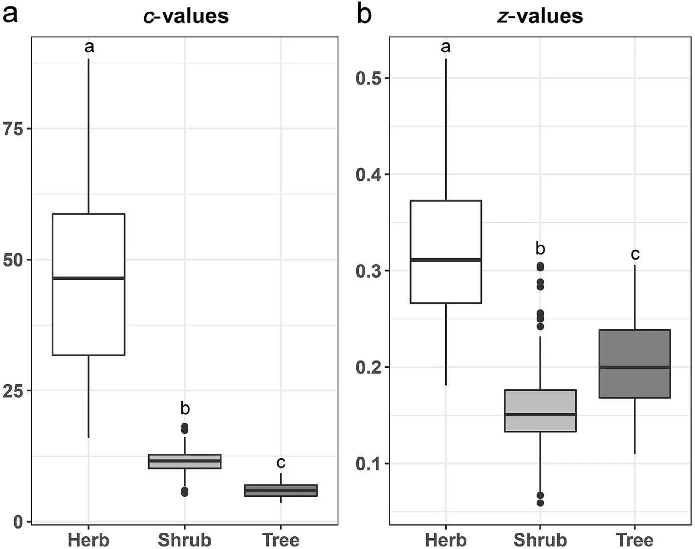
Fig.3. Boxplots of the observed parameters of the power function model(c,z-value)among the three plant life forms.The upper and lower edges of the box represent quartiles Q3 and Q1,respectively,while the middle line represents the median.The upper and lower ends of the extension lines represent Q3±1.5＊and Q1±1.5＊IQR.Different letters represent significant differences among plant life forms based on the Mann-Whitney test (P ＜0.05). (IQR: interquartile range).

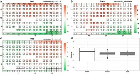
Fig.4. Patterns of standardised variation coefficient δ in the plot.(a–c)The spatial patterns of standardised δmj at the maximum sampling area Am from each sampling starting location between the three plant life forms.The numeric at the top right is the mean±sd.(d)Boxplots comparing species-area relationship(SAR)variations(standardised δmj) between the three plant life forms. The asterisk represents significant differences based on the non-parametric ranking test (P ＜0.05).

4. Discussion

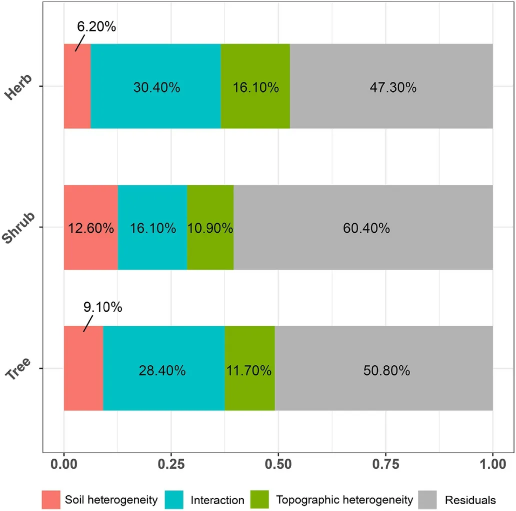
Fig. 5. Variance parititioning of soil and topographic heterogeneity effect on the variation of species-area relationship(δstandard)for different plant life forms.

Based on a comprehensive investigation in the FORESTGEO site Wanglang Plot, we investigated the variation of SARs with different sampling starting locations.We found that the SAR forms varied among plant life forms (Fig. 3), and sampling starting location affected the formats and power model parameters of the SARs(Figs.3 and 4).We further found that environmental heterogeneity was a key factor explaining the variation in SARs among the studied plant life forms and sampling starting location (Fig. 5). Most previous studies have constructed SARs based on a few sampling series data and replaced species richness in each area level with the mean richness (Meixler et al., 2019; Dengler et al.,2020; Giladi and Ziv, 2020), but ignored variation of SARs at different sampling starting locations. The environmental heterogeneity increased with the expansion of the sampling area(Davies et al.,2005;Kallimanis et al., 2008). It is important to develop a suitable sampling design to construct an accurate SAR (Ulrich and Buszko, 2007; Azovsky, 2011;Bueno et al., 2020). These findings help understand the importance of selecting sampling starting locations and environmental heterogeneity in constructing SARs.

4.1. Differences of SARs among plant life forms

The result of comparing z-values of power-law models was different from our first hypothesis. The larger z-values (steeper SARs) for the herbaceous plants compared to the trees(Fig.3)were inconsistent with Drakare et al. (2006), who suggested that SARs were flatter (smaller z-values)for smaller organisms.Some studies have reported that steeper species-area curves have a greater difference between the local species composition and regional species pool and a higher endemic species ratio(Tuomisto, 2010; Storch, 2016). In this sense, our results suggest that herbaceous plants also had dispersal limitations and were more spatially aggregative distributed than the shrub and tree species in the plot(Fig. 4). Large organisms did not always have narrower dispersal and steeper SARs than the small organisms. One possible reason is that the z-value in a power-law SAR is scale-dependent(Turner and Tjørve,2005;Pereira et al., 2012; Polyakova et al., 2016), partly because the determinants of a SAR are different between smaller and larger scales(Williamson et al., 2001; Storch, 2016). At a small scale, the number of individuals regulates the SAR, and more individuals in the community may result in a steeper SAR (McGlinn et al., 2019, 2020). In our study,herbaceous plants were more abundant than trees and shrubs, thus had larger z-values. Another possible reason is that environmental heterogeneity prevents a wider dispersal range. Small organisms, such as the herbaceous plants, had limited dispersal ability under environmental effects which led to colonizing aggressively in a micro-habitat.

4.2. Influences of sampling starting location on the SARs

The impact of sampling starting location was supported by our results.Limited by the approach to obtain large-scale sampling data,most species-area curves were derived from a few sampling series data points,rather than a comprehensive survey for the whole study region(Scheiner,2003; Meixler et al., 2019; Dengler et al., 2020), which ignored the stochasticity and variation of SARs within plots. Most of the previous studies have used the mean values to substitute observed species richness at each sampling area level and fit the species-area models with a few series data points(Kunin et al.,2018;Hobohm et al.,2019).Our results suggest that SARs should be constructed and fitted using fine-resolution sampling data, rather than coarse-resolution data, to obtain species diversity distribution patterns in detail (Steinbauer et al., 2012). A comprehensive sampling design that covers the entire survey region,for example, by selecting multiple sampling starting locations as much as possible, considering the mean and variation of SAR at the same time,setting more hierarchical series and area gradients (Drira et al., 2019;Giladi and Ziv, 2020; Dembicz et al., 2021), has a greater potential to reveal the true SAR and to decrease the effect of stochasticity.

4.3. Effect of environmental heterogeneity on SAR

The role of environmental heterogeneity was further supported.Although higher variance explained by environmental heterogeneity for herbaceous than woody plants which against our original hypnosis,because the herbaceous plant presented spatially more aggressive patterns than the woody.The similarity of plant community composition is driven by both niche and neutral processes at the fine-grain scale,and the stochastic process plays a major role in some woody community assembly mechanisms (Legendre et al., 2009; Shipley et al., 2012). However, our results indicate that the deterministic process mainly affected community assembly leading to an intense heterogeneity in the Wanglang Plot rather than stochasticity (Mori, 2019; Ning et al., 2019). Environmental heterogeneity limited the dispersal range of all individuals and shaped heterogeneous distribution patterns(Shen et al.,2009).This also proved that environmental heterogeneity directly affects the SAR formats of different plant life forms through the spatial distribution of species. A non-linear relationship was apparent between environmental heterogeneity and curve variation in plant life forms (Fig.S4–S6).

The result of variance partitioning for a single predictor showed the dominative contribution of the main environmental factors, which are slightly different among plant life forms. Topographic and soil factors affect plant life forms differently(Table S1),implying that plant life forms have specific requirements for environmental adaptation (Bimler et al.,2018;Simova et al.,2018).In our study,topographic heterogeneity, represented by variation of aspect, significantly affected SARs of the herbaceous plants, shrubs, and trees (Table S1). The aspect represents the availability of light to plants having an important influence on the community composition and spatial distribution of plant species (Punchi--Manage et al., 2013). The altitude and slope were related to the species-area curve variation of the tree species(Table S1),suggesting that the diversity distribution pattern of trees in the Wanglang Plot was affected by more complex micro-habitats changes resulting from topographic heterogeneity.The impact of soil heterogeneity mostly resulted from the energy variation(Table S1).For example,soil temperature and water content directly reflect the energy and water availability, and the distribution of trees and shrubs may be more strongly affected by the heterogeneity of hydrothermal conditions (Wang et al., 2009). Soil bulk density was important in shaping the SARs of the trees (Table S1), indicating the physical conditions to successfully establish and persist tree species (Liu et al.,2019).Soil nutrients mainly contributed to herbs(Table S1),making herbaceous competition more intense in heterogeneous than homogeneous environments(Hutchings et al.,2003;Xue et al.,2019).

It should be noted that our study demonstrates the conspicuousness of the contribution of environmental factors to the variation of species-area curves from different sampling starting locations. The correlation effect of environmental heterogeneity is inevitable with an increase in the sampling area(Keil and Chase,2019).We were not able to eliminate the collinear environmental variables and their correlations(Fig.S7). However, our study helps to understand the impact of environmental heterogeneity on the construction of SARs and suggests to minimise this impact as much as possible or take it into full consideration,especially in a heterogeneous habitat with unrandom distribution patterns of species.

5. Conclusion

Our results demonstrate that all plant life forms within a plot have specific spatial distribution patterns, which shape the general form of SAR.The sampling starting location affects the variations in SAR,which is partly due to environmental heterogeneity. However, the main environmental factors slightly vary among plant life forms. In conclusion,environmental heterogeneity influences the SAR curves through the spatial distribution of species. The construction of a SAR based on the mean species richness with a few sampling series data points has the weakness of stochasticity.Hence,we recommend considering the design of sampling starting location when constructing SAR curves,especially in a heterogenous habitat with unrandom distribution patterns of species.

Funding

This work was supported by the National Natural Science Foundation of China(Nos.31988102 and 31300450).

Availability of data and material

The data of estimated c, z-values of power model SARs originated from different quadrates between three plant life forms is available as supplementary data in the excel Supplementary Data.

Authors’contributions

J.Z. conceived and designed the study. C.H. and L.F. performed the data analysis. X.X., F.F., Y.L., L.F. and L.H. conducted field work. S.L.setup the study plot. C.H., X.S., S.L., C.J. and J.Z. discussed the results,C.H. and L.F.drafted the manuscript,with input from all authors.

Ethics approval and consent to participate

Not applicable.

Consent for publication

Not applicable.

Competing interests

The authors declare that they have no conflict of interest.

Acknowledgements

This work was supported by the National Natural Science Foundation of China (Nos. 31988102 and 31300450). We declare no conflict of interest.We are also grateful to the anonymous reviewers and the handling editor for their insightful and constructive comments which improved the manuscript.

List of abbreviations

Species-area relationship:SAR

Appendix A. Supplementary data

Supplementary data to this article can be found online at https://do i.org/10.1016/j.fecs.2022.100033.