Cross-classes domain inference with network sampling for natural resource inventory

Zhngyng Hou, Ronl E. MRorts, Chunyu Zhng,＊, G¨orn Ståhl, Xiuhi Zho,Xujun Wng, Bo Li, Qing Xu

a The Key Laboratory for Silviculture and Conservation of Ministry of Education, Beijing Forestry University, Beijing, China

b Department of Forest Resources, University of Minnesota, Saint Paul, MN, United States

c Department of Forest Resource Management, Swedish University of Agricultural Sciences, Umeå, Sweden

d Office of the National Forestry and Grassland Administrations Forest Resources Supervision Commissioner in Beijing, Beijing, China

e Department of Statistics, University of Illinois at Urbana-Champaign, Champaign, IL, United States

f Key Laboratory on the Science and Technology of Bamboo and Rattan, International Centre for Bamboo and Rattan, Beijing, China

Keywords:Cross-classes domain estimation Design-based inference Network sampling Generalized systematic adaptive cluster sampling Forest inventory

ABSTRACT

1. Introduction

Survey sampling provides ecosystem ecology and natural resource management with reliable information,much of which is used to estimate parameters for biotic and abiotic variables of biodiversity, dynamics,competition,energy and material cycling,not just at the population level,but also at the domain level (Margules and Pressey, 2000; Williams and Brown,2019).The term domain denotes a subpopulation,that is,a subdivision of a (spatial) population according to a quantitative or qualitive condition of interest (COI) (Rao and Molina, 2015). While population inference aims to estimate parameters such as the total or mean of the variableofinterest(VOI)fortheentirepopulation,domaininferencedoesso for a target domain,such as a county domain of a province population or a speciesdomainofavegetationoranimal population.Domainestimatesmay reflect the gradient, distribution, and structure of a VOI, thus enriching present knowledge, future projection, and decision-making for natural resource management.

There are two distinct types of domains, design- and cross-classes domains(Kish,1980).Design domains refer to the domains of a population which are not crossed or intersected with each other,and the set of which comprises the complete population,e.g.,county domains of a province or state population,stratum domains of a forest population(Purcell and Kish,1979). Separate samples with possibly separate sampling designs are selected for each domain,and their combination forms the entire sample from which the population estimate is usually calculated as a weighted sum of respective within-domain sample-based estimates (Chambers and Clark,2012).The literature pertaining to design-domain problems is rich and comprehensive and is typically found under the topic area of small-area estimation and stratified sampling (S¨arndal et al., 1992; Rao and Molina,2015). For either a direct or indirect domain estimation, examples include model-based composite estimators and synthetic estimators(Ghangurde and Singh,1978;Schaible,1978),design-based stratified estimators, generalized regression estimators and the hybrid calibration estimator(Lehtonen and Veijanen,2009,2019).These estimators,except the stratified estimators,depend on models and require domain sampling frames and auxiliary data that are clear and readily available.

In natural resource inventory, however, most classes listed in the condition tables of national inventory programs are characterized as crossclasses domains; examples for the Forest Inventory and Analysis (FIA)program of the U.S. Forest Service include vegetation types, productivity classes,and age classes(FIA,2021).To date,challenges remain active for cross-classes domain estimation because sampling frames and spatial distributions of the domains are generally unknown. This would make a model-dependent procedure inefficient because modeling requires explicit domain locations for observing unit-or area-level auxiliary data(Rao and Molina, 2015). Hence, cross-classes domain inference relies mostly on design-based sampling with respect to the entire population as opposed to just the domain, with multiple related challenges: (1) efficient sampling strategies are difficult to develop because of little priori information about the target domain; (2) a sampling design for a particular domain would create imbalances for other domain samples and the population sample for multiple VOIs; (3) domain inference relies on a sample designed for the population, within-domain sample sizes could be too small to support a precise estimation;and(4)increasing sample size for the population does not ensure an increase to the domain, so actual sample size for a target domain remains highly uncertain,particularly for small domains.

Systematic sampling(SYS)has been used for population and both types of domain inferences, with a long history of serving official reporting instruments in different sectors around the world.The Nordic countries,the USA, China, and many other countries have established their respective national forest inventory (NFI) programs based on variations of SYS(Tomppo et al.,2010;Vidal et al.,2016).Compared with simple random sampling (SRS), SYS is usually more precise and more convenient in logistics than to measure an equal number of plots selected at random(Heikkinen,2006).Importantly,the spatially balanced systematic sample benefits NFIs in that it serves as a common sample appropriate for inventorying multiple VOIs instead of just one. Because of annual sample plots of 4,400 to 15,000 in the Nordic countries and 1,200 to 3,500 in individual American states(Hou et al.,2021),cost-efficiency relative to the tradeoff between reducing variance and increasing sample size is key to field campaigns at this scale. However, increasing sample size for SYS would remarkably increase the number of sample plots and thus is not always feasible (Thompson, 2012; Hou et al., 2015). Therefore,cost-efficient alternatives,preferably compatible with SYS,must be sought.

The design-based network sampling is a viable option. Named by Thompson and Seber (1996), network sampling dates to Sirken (1970,1983)with Chaudhuri’s(2000)exposition based on the foundation laid by Thompson(1990,1992)and Thompson and Seber(1996);Rao(1999)also elaborated on this topic.Networking and adaptiveness are two grand features attributed to network sampling,as demonstrated in Section 2.2.1 for spatial sampling and in Section 3 for regional scale examples.Unlike SYS or otherconventionaldesign-basedsamplingapproacheswhoseestimatorsare based on unit-level observations, estimators used with network sampling are based on network-level observations.Adaptiveness refers to networking contingent on the COI,neighborhoods and an initial sample selected with a conventional design, leading to the final sample in the form of networks grown out of the initial sample.However,most network sampling procedures, such as the adaptive cluster sampling (ACS) with the initial sample selected by SRS(Thompson,2012,Chapter 24)and the systematic adaptive cluster sampling(SACS)with the initial sample selected by SYS(Thompson,2012, Chapter 25), were devised for inventorying rare VOIs, except the generalized SACS (GSACS) which was devised for inventorying general VOIs(Xu et al.,2021).Instead of adding sample units to the initial sample,GSACS works in reverse by removing sample units from the initial sample,and thereby solves SACS problems of oversampling,uncertain sample form,and sample imbalance for alternative VOIs.GSACS is compatible with SYS and does not necessarily modify NFI field protocols or designs.

Consequently,theobjectivesofthisstudyarefivefold:(1)toproposeand illustrate network sampling with GSACS for inventorying cross-classes domains; (2) to derive Hansen-Hurwitz (HH) and Horvitz-Thompson (HT)estimators for use within GSACS for domain totals; (3) to analytically compareestimators withinGSACS andwithSYS;(4)toempiricallycompare the sampling distributions of the respective estimators; (5) to summarize rules of thumb with respect to design strategies for variance reduction.

2. Sampling designs and estimators

2.1. Systematic sampling (SYS)

SYS,as thoroughly detailed in Thompson(2012,Chapters 12 and 25),is the basis for GSACS which was devised particularly for inventorying cross-classes domains in Section 2.2. Consistent with Thompson (2012,p.158),Fig.1 illustrates a typical SYS design for a spatially rectangle area of interest containing a forest compartment.

The rectangle area is firstly tessellated with population units of a given size and shape,for example,a square in the Chinese NFI system.The population of these units is then partitioned into primary sampling units(PSUs)such that each PSU consists of a collection of secondary sampling units(SSUs) regularly spaced over the area. Subsequently,a sample is selected from the collection of PSUs, although actual measurements are made on SSUs.Because the sample is randomly drawn from the collection of PSUs,the population size,N,denotes the total number of PSUs,and the sample size,n,denotes the number of selected PSUs;M denotes the total number of SSUs in a PSU;thus MN is the total number of population units.In practice,the key is that whenever any SSU of a PSU is included in the sample,all the SSUs of that PSU are included,too(Thompson,2012,p.157).

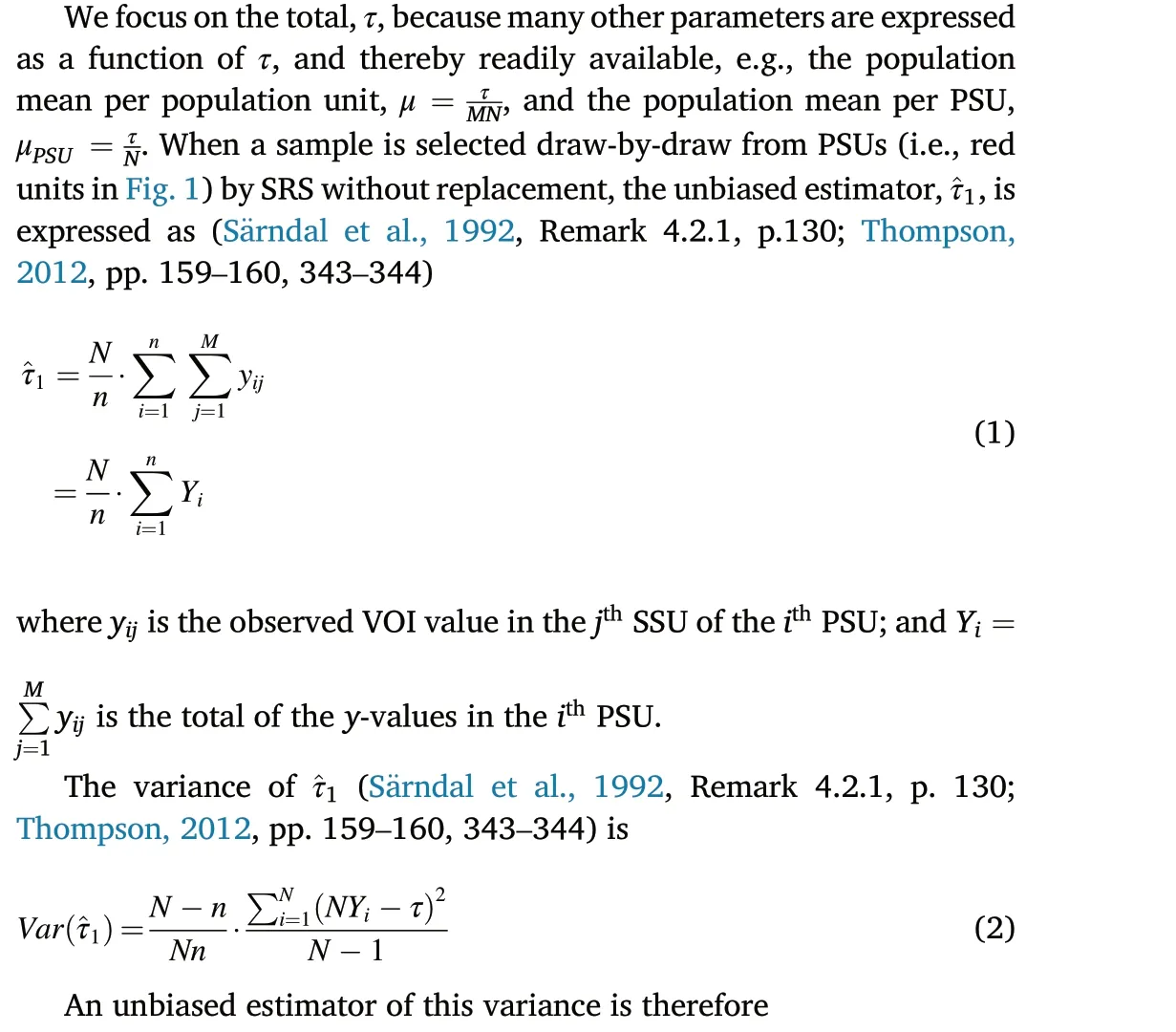
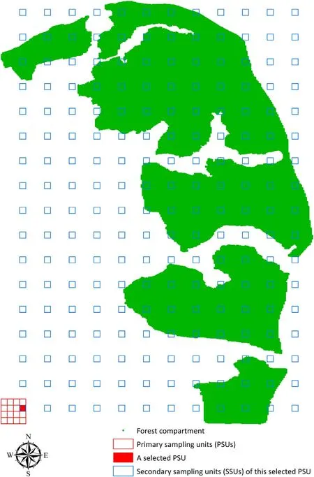
Fig. 1. Demonstration of partitioning into primary and secondary sampling units for systematic sampling.

To prevent ambiguities with simple random cluster sampling (SIC),characteristics underlying SYS are stressed. First, SYS and SIC share the same estimators above(Thompson,2012,Chapter 12).Although they seem on the surface to be opposites,one spacing out the sampling units and the other bunching them together,the two designs are of the same structure.Either case, because every SSU is observed within a selected PSU, the within-PSU variance does not enter Eq.(2)or Eq.(3).Although SIC is likely to be inefficient for homogeneous clusters, it is usually much cheaper to survey clusters of units than to survey spatially scattered SYS units.Second,the SYS variance above is design-unbiased,as clarified by Remark 4.2.1 in S¨arndal et al. (1992, p. 130) and Chapter 12 in Thompson (2012, pp.159–160).SYS variance just has one term that takes among-PSUs variance into account.Third,for SYS,we in principle can dispense with the notion of the SSUs and regard the PSUs as the sampling units and then use the total of the y-values of the SSUs within it.Thereby all properties of estimators are obtainable with the design by which the sample of PSUs is selected.

2.2. Generalized systematic adaptive cluster sampling (GSACS)

2.2.1. Network sampling design

GSACS was enlightened by Thompson’s statement about SACS: “A neighborhood could, in fact, consist of a set of noncontiguous units,spread out, for example, in a systematic grid pattern about the original unit(Thompson,2012,p.341).”Thorough SACS design descriptions and terminologies GSACS follows are available in Thompson(2012,p.339).

With GSACS,the systematic sample selected in Section 2.1 is used as an initial sample for providing priori unit locations from which networks are formed according to a clearly defined neighborhood and a COI, C.This C specifies a domain for estimation, and thus is the key to constructing inferences for cross-classes domains,elucidated in Section 2.5.Because the priori unit locations now become readily known, simple means such as remote sensing or a field visit without requiring major field sampling efforts work for the assessment against C.

A GSACS sample is formed in a recursive manner such that every single unit in the initial sample is a seed to be checked against C. The neighbor of a seed is spatially separated or disjoint, constrained to be a sampling unit to the left,right,top and bottom following the systematic pattern identical to the initial sample.If C is met,respective neighbors of this seed are evaluated as well. A valid neighbor is then included with that seed in the same network and treated as a new seed for another iteration of this process.This recursive process exhaustively searches and grows towards other units permissible under the constraints of neighborhood and C, and stops automatically when all PSU-intersected networks are included in the GSACS sample. Thereby, SSUs in the initial sample not meeting C are adaptively removed from an inventory. In practice,subject to a domain of interest,this assessment against C can be done in various ways that are less costly than surveying the entire unit.

The design procedures of GSACS essentially achieve a transformation from disparate units to connected networks(Thompson and Seber,1996).From the perspective of network sampling: (1) a population constitutes networksinstead of units,and GSACSpertainstosampling the population of networks rather than the population of units;(2)a network is intersected by onlyonePSU,i.e.PSU-specific,indicatingthattheSSUsofaPSUcomprisethe poolforallnetworksspecifictothisPSUtotakeform;(3)GSACSonlyrequires the locations of the initial SYS sample but does not have to require a SYS sample observed in the first place;(4)unit locations in the initial systematic sample arethepoolfromwhichGSACSnetworksareformed,indicatingthat thesenetworkscanonlygrowfromtheinitialsample;(5)networksmaytake different forms based on the same initial sample,subject to C(Fig.2)which facilitates constructing inferences for multiple cross-classes domains from a single common initial sample,a useful feature for monitoring different domains based on collected data such as FIA database; and (6) only network-level observations enter the GSACS estimators, indicating that non-networked units in an initial sample do not require observation.

2.2.2. Derivation of estimators

Consistent with network sampling procedures in Thompson (1991,2012), we derived both Hansen-Hurwitz (HH) and Horvitz-Thompson(HT)estimators for use within GSACS.The HH-estimator takes the form

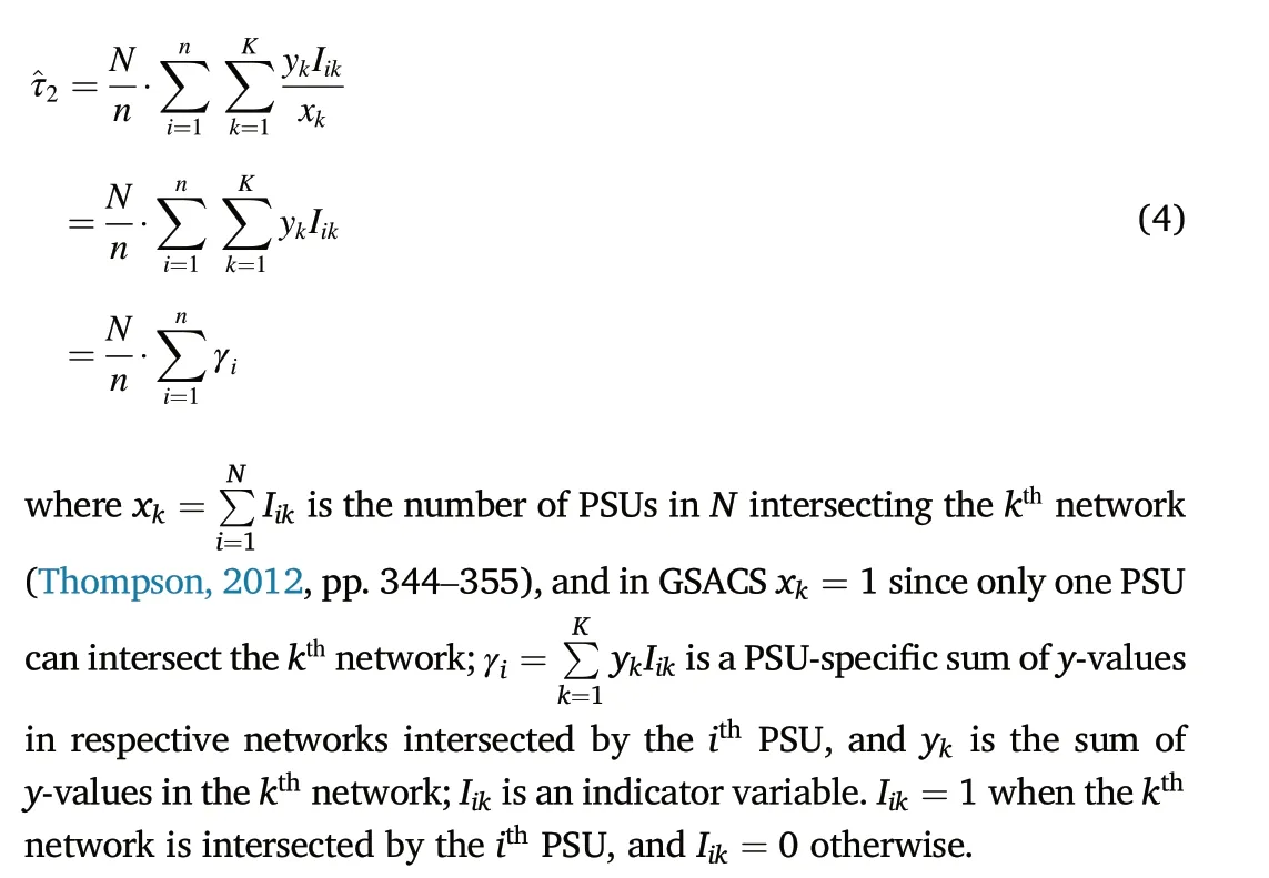
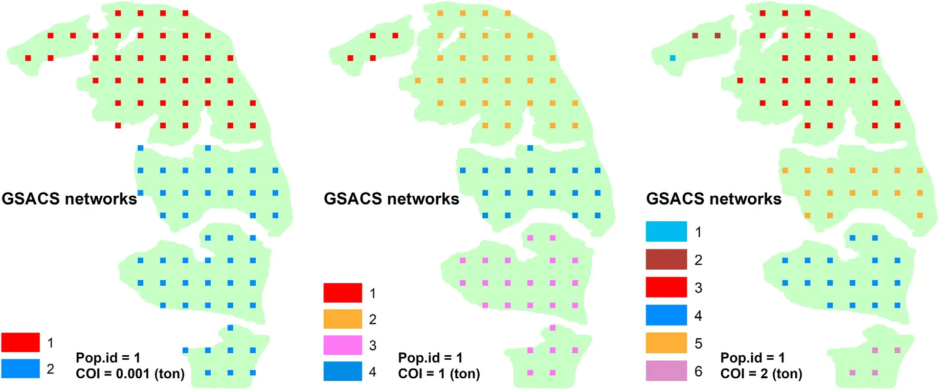
Fig.2. Formation of GSACS networks subject to COI for carbon inventory.Pop.id is the Population ID listed in Table 1;COI specifies a cross-classes domain for estimation.A domain comprises sampling units whose carbon values in metric ton are equal to or larger than COI,so domain estimates reflect the gradient of carbon as COI increases.

Because^τ2is the sample mean of the Nγifor a simple random sample of size n, the variance of ^τ2follows from the usual results on simple random sampling(Thompson,1991,Appendix A),obtained readily as

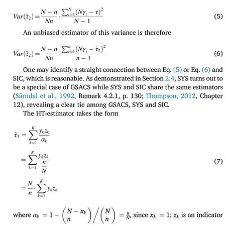
where E（zk）=αkand E（zkzj） =αkj.Note there are two circumstances for the joint probability, αkj, in GSACS: for networks k， j ∈same PSU,

2.3. Connections within GSACS estimators

Interests exist in comparing the two types of GSACS estimators,because differences in their efficiency and behavior would translate to cost spent on and reliability obtained from an inventory.Surprisingly,the two point estimators are equivalent in use,i.e.

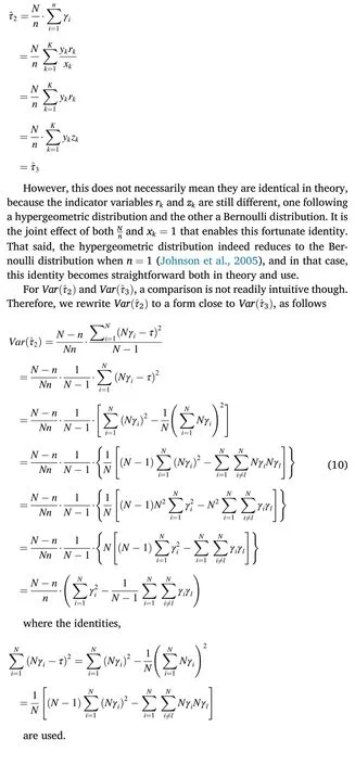
Comparing Eq. (10)and Eq.(8) analytically,we reach four findings.First,Var（^τ3）=Var（^τ2）holds valid when in a PSU there exists only one network, i.e., K = N, by canceling the second variance component of Var（^τ3）.Second,the advantage of Var（^τ3）is that ^Var（^τ3）works for n =1,whereas ^Var（^τ2）does not.Third,the first two findings are essentially two extreme situations for Var（^τ3）,canceling respectively the second or third variance component of Var（^τ3）. Fourth, other situations for Var（^τ3） are somewhat between the first two, requiring empirical comparisons for Var（^τ2）and Var（^τ3）with sampling simulations,as done in Section 3.

2.4. Connections between GSACS and SYS estimators

Interestingly,the SYS estimators in Section 2.1 turn out to be a special case of the GSACS estimators when the condition of interest C is released to be null and void, so that the domain becomes the entire population.Then,

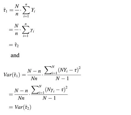
2.5. Cross-classes domain inference with GSACS

GSACS is adaptive sampling that takes advantage of networking initial sample units for making an inference.Networking is subject to C,which can be descriptive, qualitive, quantitative or even null and void,functioning as a domain-specifier. Based on the initial sample, C adaptively adjusts the formation of networks enroute to an inference about the domain parameter specified by this C; and as C changes from one to another,the domain-specific estimate changes in tandem.

GSACS is highly flexible,suitable for inventorying both a population and a domain.For population inference,GSACS reduces to SYS,because SYS is a special case of GSACS subject to C being null and void.In effect,this conditioning makes networking unconditional such that all units in the initial sample are members of one common network.As a result,the samples for GSACS and SYS become identical,and as analyzed in Section 2.4, the point and variance estimators are equally efficient for both GSACS and SYS.

For domain inference, GSACS works for both the design and crossclasses domains. For design domain, C can specify a region or stratum in a population, e.g., a county in a province or state. Then, only units belonging to this county in the initial systematic sample are networked so that the estimation is only with respect to the appointed county. For a cross-classes domain, C can specify a VOI class in a population, e.g.,productivity class, by operating as a cutoff threshold (Thompson, 2012,p. 347). Such a class or domain comprises sampling units whose VOI values are equal to or larger than C.

In this study, we focus on inventorying cross-classes domains with GSACS. For simplicity, a cross-classes domain refers to a VOI class defined by C.Such a domain comprises sampling units whose VOI values are equal to or larger than C,and the inference is about the domain total of this VOI.As detailed in Section 3,the VOI in our sampling simulations for evaluating the sampling distributions of respective estimators is aboveground(ABG)carbon stock in metric tons.As illustrated in Fig.2,when C =0.001 ton, all units in the initial sample which meet this condition by having ABG carbon equal to or larger than 0.001 ton are networked,and then used for estimating this domain-specific total;when C=2 ton,the total of this domain is estimated in the same way,which should be less than for the aforementioned class. Likewise, we can inventory a sequence of carbon stock classes with not only the point estimates, but also the variance estimates available, from a common initial sample. These domain estimates reflect the gradient, distribution, and structure of ABG carbon in a population,and compared with SYS devised primarily for inventorying a population,GSACS enriches inferences,and thus knowledge,with respect to both the population and domains.

3. Monte Carlo simulations

3.1. Sampling distributions for validation and comparison

Validation and comparison within GSACS and between GSACS and SYS were conducted using Monte Carlo sampling simulations involving three steps.First,construct an artificial population mimicking a real one,so that the parameters of the artificial population are readily known for the population and domains. Second, draw a sample following a prescribed design and use it for estimation.Third,iterate the second step.

3.2. Artificial populations

We generated 16 artificial populations based on real data collected from eucalyptus plantations in Hainan,China.In a population,each tree occupies 5 m2on the ground and all trees form a systematic lattice with known coordinates and attributes including diameter, height, stem volume, ABG biomass and ABG carbon (Fig. 1). Allometric models and diameter distributions were used for generating these attributes, with procedures detailed in Hou et al.(2015)and Xu et al.(2021).

Because the VOI value associated with a tree would eventually diminish to zero upon the death of this tree,tree mortality can be used as the surrogate for any VOI that relies on living status in the investigation of spatial effects on sampling. In other words, investigating the spatial effects of a VOI is equivalent to investigating the spatial effects of tree mortality. Mortality (%) specifies the prevalence of a pattern, and the cluster diameter in meters expresses the range of spatial autocorrelation.All trees inside a cluster are dead,and a dead tree’s VOI is set to zero.

In this study,respective populations exhibit different spatial patterns that are either random or clustered, as summarized in Table 1, and visualized in Figs. 1 and 3. The VOI is ABG carbon stock, with spatial patterns generated using the DNR Sampling Tools operating on tree coordinates (DNR, 2021). With this comprehensive set of populations,practitioners gain clear insight into the behavior of GSACS when applied in practice to inventorying cross-classes domains.

3.3. Design strategy

Design plays a role in the selection of a sample and forms the basis for making an inference. An ideal design helps to increase inferential precision with a relatively small sampling intensity where sampling intensity refers to the sample area as a percentage of the entire area,a key factor influencing the cost of field campaigns. The sample area is expressed as the product of the 20 m×20 m plot size and the number of sample plots comprising the sample.

The number of plots in a sample is determined by partitioning the population into PSUs as explained in Section 2.1. Two PSU strategies were compared,one of size N =16(4 by 4 PSUs,i.e.,the red squares in Fig. 1) and the other N =64 (8 by 8 PSUs), leading respectively to sampling intensities of（6.25×n）%and（1.56 ×n）%,as n increases from 1 to N for the selection of an initial sample.This partitioning emphasizes the comparability across sampling intensities, with other conditions being equal.Although the initial sample was selected following SYS andthen networked for GSACS estimation, in practice, GSACS does not require initial observation of all sample plots because C deletes nonnetworked plots in the initial sample from observation.

Table 1 Populations generated for sampling simulations.

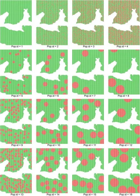
Fig. 3. Visualized populations generated for sampling simulations, with living trees in green, and dead trees in red. (For interpretation of the references to colour in this figure legend, the reader is referred to the Web version of this article.)

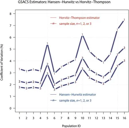
Fig. 4. Identical efficiency for GSACS Hansen-Hurwitz and Horvitz-Thompson estimators, illustrated with N =64 at C = 0.001.

4. Results and discussion

4.1. Comparison within GSACS estimators

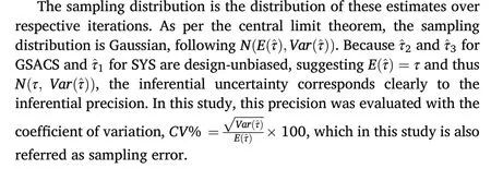
As expected,the point estimates for the GSACS HH-estimator and the HT-estimator (^τ2vs ^τ3) are identical. Unexpectedly, their variances are also identical,as depicted in Fig.4.It turns out that both GSACS HH-and HT-estimators are equivalent,with Var（^τ3）being a decomposed Var（^τ2）via networks, and with Var（^τ2） being an aggregated Var（^τ3） via PSUs.Since both estimators are equivalent, the rest of our analyses regards them interchangeably.

Importantly,a design-unbiased variance estimator is now found for a single systematic sample.The major advantage of Var（^τ3）is that ^Var（^τ3）works for n =1,whereas ^Var（^τ2）does not.The interests exist in that(1)^Var（^τ3）works for an initial systematic sample of size one and more,while^Var（^τ2）just work for that of size two and more;and(2)because SYS is a special case of GSACS, ^Var（^τ3） works for SYS of a single systematic sample,suggesting that a design-unbiased variance estimator for a single systematic sample is found readily available.

4.2. Comparison between the GSACS and SYS estimators

Consistent with Section 2.4, the estimates for GSACS and SYS are identical at the population level, indicating that SYS is a special case of GSACS.Table 2 presents a comparison between GSACS and SYS for their sampling distributions in the form of sampling errors.As shown,GSACS is more efficient than SYS, because with fewer observations, GSACS is equally precise and applies wherever SYS applies. While the sampling errors are identical, the sampling intensity is remarkably smaller for GSACS,on average 40%of that for SYS for N =64 and 20%for N =16.

Table 2 Efficiency comparison between GSACS and SYS estimators,with GSACS at C =0.001.Intensity refers to the sampling intensity,and CV the coefficient of variation or sampling error.

Both C and the networked units as the basis for inference contributed to this interesting result above. Specifying C to be a reasonably small value, such as C = 0.001, is analogous to C=0 whereas it creates a collateral effect that the actual number of networked sample plots requiring observation is many fewer than when using C = 0.This minor tweaking leads to little difference in estimation but contributes to substantially reducing the number of initial sample units requiring observation.

Although sample size can be increased to reduce variances for both GSACS and SYS, the increase in sampling intensity to achieve the same reduction is much smaller for GSACS than for SYS. Network sampling pertains to selecting a sample of networks from a population of networks,but SYS pertains to selecting a sample of units from a population of units(Chaudhuri, 2015). Non-networked units in the initial sample are not used with the GSACS estimator and thus are excluded from fieldwork,whereas in SYS, every sample unit is used with the SYS estimator and thus must be observed in the field,with no exception(Thompson,2012).These excluded plots are quantitatively expressed by the difference between sampling intensities for SYS and GSACS in Table 2, and visually between Figs.1 and 2.

Because sampling errors increase as spatial aggregation increases,GSACS and SYS are found both sensitive to spatial effects. However, a useful finding is that the GSACS sampling intensity decreases as the spatial aggregation increases, which is consistent with Xu et al. (2021).This means that fewer sample plots are needed for aggregated populations, or equivalently, sampling errors can be further reduced by increasing the GSACS sample size without increasing the cost initially budgeted for SYS.For example,with Pop.id=16,SYS observed 1.56%of the population for a sampling error of 15.12%, but GSACS attained a smaller sampling error of 10.61% by only observing 1.15% of the population (Table 2). Reasonably, GSACS would be more efficient for field campaigns, and thus interesting for constructing field observation networks to which expensive monitoring devices are deployed and maintained at appointed locations(FIA, 2021).

4.3. Cross-classes domain inference

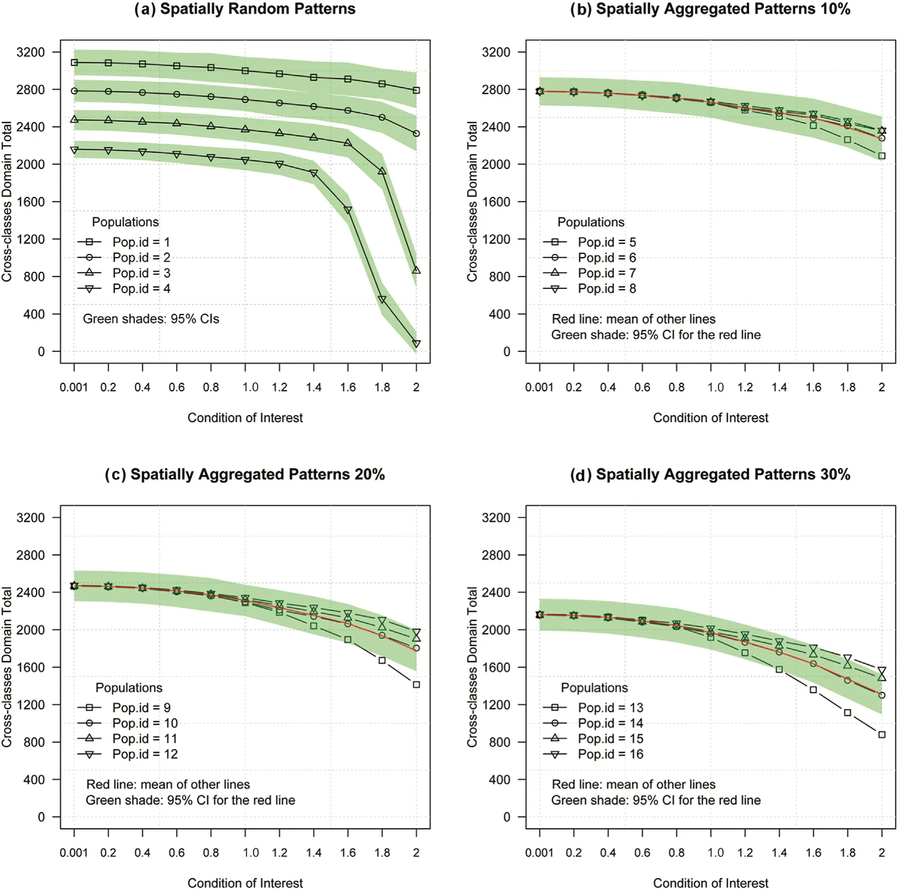
Fig. 5. GSACS reveals the gradient, distribution, and structure of carbon pools for 16 populations following different spatial patterns. Herein, N = 16 and n = 2.

Fig. 6. GSACS requires fewer sample plots for observation as the domain size decreases. Herein, N =16 and n = 2.

GSACS has the advantage of being universal in making both population and domain inferences, with results for the latter summarized in Figs.5 and 6.Although ABG carbon was used for demonstration,the VOI can be generalized to other variables without impairing analyses regarding the behavior of GSACS. Four findings are relevant: (1) in respective populations, GSACS captured the variability between domains;(2)as the domain size decreases,the number of plots required for observation decreases,but the sampling error increases,consistent with Kish (1980); (3) the domain size decreases faster for random patterns than for aggregated patterns;and(4)given a domain,the sampling error is smaller for random patterns than for aggregated patterns,and smaller for less aggregated than for more aggregated patterns.

Precise estimation for large cross-classes domains is less of an issue than small and mini domains. With non-network sampling procedures such as SYS, although increasing the sample size, n, is effective for reducing the sampling error for small and tiny domains, this solution is too expensive to be considered even for design domains (Hou et al.,2021), let alone cross-classes domains. However, with the network sampling of GSACS, increasing n for small and mini domains is feasible and efficient because the actual measurements are made on member units only.As shown in Fig.6,the sampling intensity for GSACS at n=2 for C=2 just took 4%of the maximum compared to 12.5%if SYS were used. For mini and rare domains, adaptive cluster sampling, systematic adaptive cluster sampling, and stratified adaptive cluster sampling can also be considered because inventorying rare attributes is analogous to inventorying these domains for which these network sampling procedures were devised(Thompson,2012).

4.4. Effects of primary units

An ideal design contributes to decreasing the sampling error with a relatively small sampling intensity. Two PSU strategies were compared,one of size N =16 (4 by 4 PSUs) and the other N =64 (8 by 8 PSUs),leading respectively to sampling intensities of （6.25×n）% and （1.56 ×n）%, as n increases from 1 to N for selecting an initial sample. While these sampling intensities apply directly to SYS, they are smaller for GSACS(Table 2,Fig.7).

Three findings are relevant.First,it is explicit that the PSU strategy is a factor that matters in reducing sampling error for GSACS and SYS.Second, sampling intensity is more indicative than n in comparisons across different designs. Although the sampling error seems smaller for the PSU design of N =16 than N =64 at n =1,the sampling intensity is only 1/4 for the latter (Fig. 7). Third, we recommend the PSU strategy with N and n being both large, rather than both being small. The sampling error for the PSU design with N =16 at n=1 is about the same for the PSU design with N =64 at n = 4, and this correspondence remains valid as n increases,regardless of C or spatial patterns(Fig.7).

Fig. 7. Effects of primary units on sampling errors, with C = 0.001. Similar result pattern applies to GSACS as C increases.

The third finding is a rule of thumb important for both GSACS and SYS.With this PSU strategy,practitioners can work around the paradox of missing design-unbiased variance estimators for SYS at n = 1,instead of compromising with alternative variance estimators like one for simple random sampling or one that is biased(Wolter,1984;Magnussen et al.,2020). In this regard, incidentally, the GSACS HT-estimator appears promising for SYS at n =1,i.e.,single systematic sample,which deserves further research in a separate study. Hou et al. (2015) and Xu et al.(2021)investigated the size effect of SSUs,i.e.,sample plots,on sampling errors,with a conclusion that smaller SSUs should be employed.Jointly with their conclusion,the sampling error effectively decreases as N and n increase,and meanwhile, as SSU size decreases.

4.5. Effects of spatial patterns

Spatial effects reside in the distribution of VOI values across sampling units and is characteristic of a spatial population.The response paradigm for different spatial effects reflects the efficiency and robustness of the sampling procedure,and thus is the basis for formulating a rule of thumb that practitioners can use to reduce sampling error and cost. These paradigms are summarized and depicted in Fig.8.

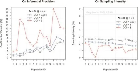
Fig. 8. Response pattern to respective populations on behalf of different spatial effects.

Three findings are relevant. First, spatial effects explicitly affect the sampling error and intensity,both at the population(i.e.,C =0.001)and domain levels(i.e.,other C s).Second,the sampling error increases as the prevalence of a spatial pattern increases, and the rate of increase is greater for aggregated patterns than for random patterns.This response is increasingly prominent as domain size decreases.Similar results apply to spatial autocorrelation but with fluctuations in consistency. Third, the sampling intensity decreases as domain size decreases, and the rate of decrease is greater for random patterns than for aggregated patterns.However,for small domains(e.g.,C =2),sampling intensity increases as spatial autocorrelation increases. These findings reiterate the assertion on increasing N and n, and meanwhile, decreasing SSU size as a countermeasure to neutralize spatial effects.

5. Conclusions

Eight conclusions are relevant. (1) While both the GSACS HH- and HT-estimators are unbiased with identical efficiency,the latter works for the sample size being n = 1. (2) SYS is a special case of GSACS, with estimators being equivalent for constructing inferences at the population level. Yet, GSACS is more efficient than SYS, because with fewer observations,on the order of only 20%–40%for SYS,GSACS is equally precise and applies wherever SYS applies. (3) GSACS HT-variance estimator is design-unbiased for a single SYS sample.(4)GSACS is efficient for small and mini cross-classes domains by increasing sample size without substantial increase in sampling intensity, indicating that valid data on a target domain are increased at a low cost. This is because observations used by the GSACS estimator are only obtained for networked units rather than the entire initial sample. Precise estimation for large crossclasses domains is less of an issue, though. (5) GSACS circumvents the conflicts arising from design imbalance with respect to a population or domain, because the initial systematic sample is a common ground bridging both inference levels. GSACS is readily compatible with NFI programs and ecological observation networks established with SYS.(6)Sampling error for GSACS or SYS decreases as the secondary unit size decreases down towards a tree, and as the population size and sample size increases, which is the rule of thumb for design optimizations with respect to the initial sample. (7) Sampling error increases as the prevalence of a spatial pattern increases,and the rate of increase is greater for aggregated patterns than for random patterns. This response is increasingly prominent as domain size decreases. (8) Inventorying a mini domain is analogous to inventorying a rare VOI,and thus as alternatives to GSACS, other network sampling procedures such as adaptive cluster sampling, systematic adaptive cluster sampling, and stratified adaptive cluster sampling are procedures readily available for the purpose of inventorying cross-classes domains.

Declaration of competing interest

The authors declare that they have no known competing financial interests or personal relationships that could have appeared to influence the work reported in this paper.

Acknowledgements

This work was supported by(1)the Fundamental Research Funds for the Central Universities(Grant No.2021ZY04),(2)the National Natural Science Foundation of China (Grant No. 32001252), and (3) the International Center for Bamboo and Rattan(Grant No.1632020029).