
Gelfand-Shilov Smoothing Effect for the Radially Symmetric Spatially Homogeneous Landau Equation under the Hard Potential γ=2
2022-06-21 07:28:44LIHaoguangandWANGHengyue
LI Haoguangand WANG Hengyue
School of Mathematics and Statistics, South-Central University for Nationalities,Wuhan 430074,China.
Abstract. Based on the spectral decomposition for the linear and nonlinear radially symmetric homogeneous non-cutoff Landau operators under the hard potential γ=2 in perturbation framework,we prove the existence and Gelfand-Shilov smoothing effect for solution to the Cauchy problem of the symmetric homogenous Landau equation with small initial datum.
AMS Subject Classifications:35B65,35E15,76P05.
Key Words: Gelfand-Shilov smoothing effect; spectral decomposition; Landau equation; hard potential γ=2.
1 Introduction
In this work,we consider the spatially homogeneous Landau equation
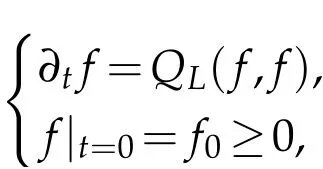
wheref=f(t,v) is the density distribution function depending on the variablesv∈R3and the timet≥0. The Landau bilinear collision operator is given by

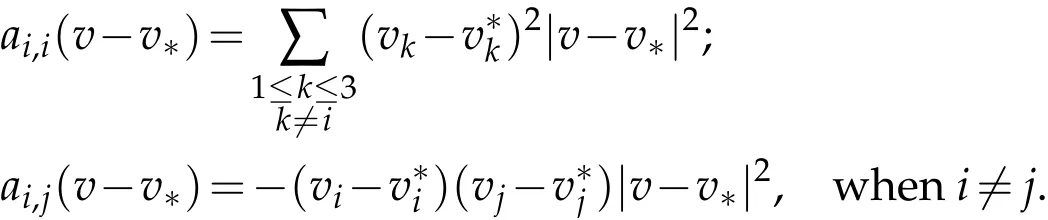
wherea=(ai,j)1≤i,j≤3stands for the nonnegative symmetric matrix

This equation is obtained as a limit of the Boltzmann equation, when all the collisions become grazing. See[1,2]. We shall consider the Cauchy problem of radially symmetric homogeneous non-cutoff Landau equation under the hard potential caseγ=2 with the natural initial datumf0≥0

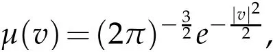
Consider the fluctuationnear the absolute Maxwellian
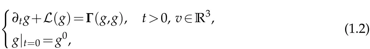
the Cauchy problem is reduced to

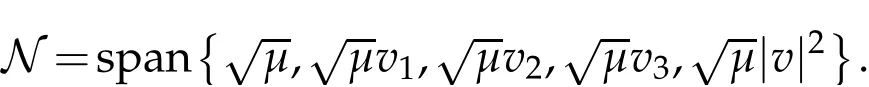
The linear operator L is nonnegative with the null space
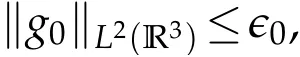
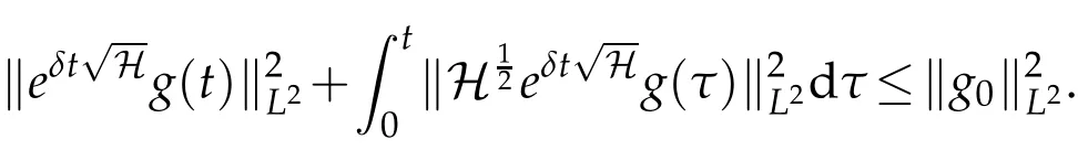
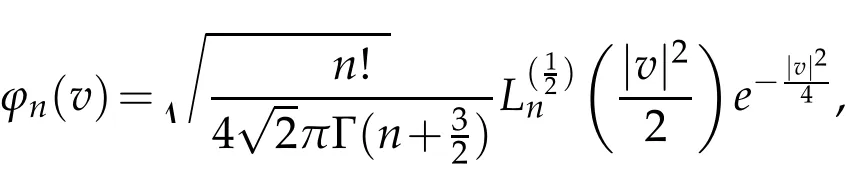
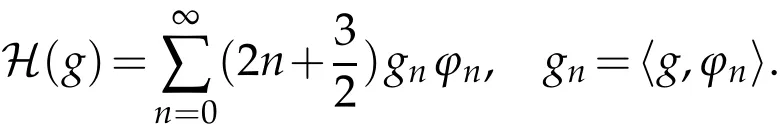
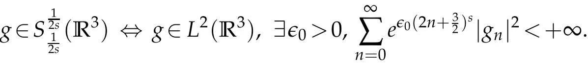
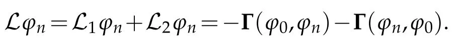
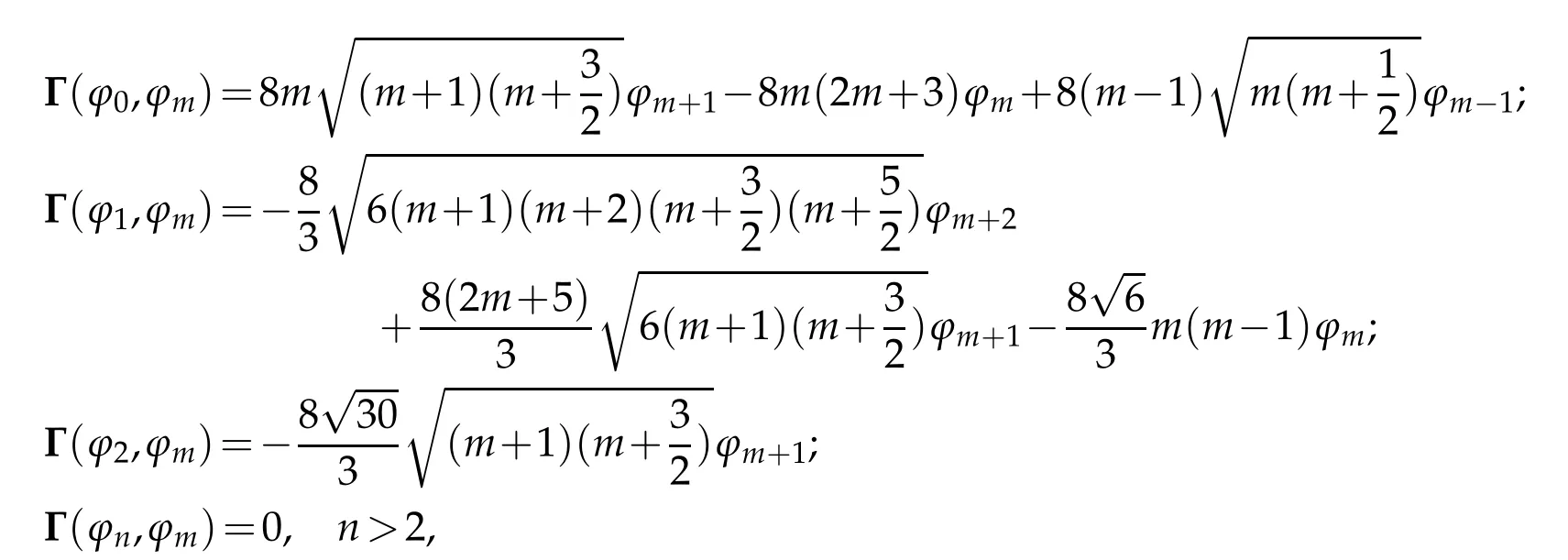
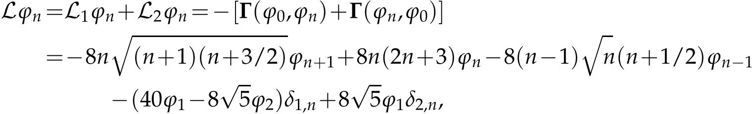
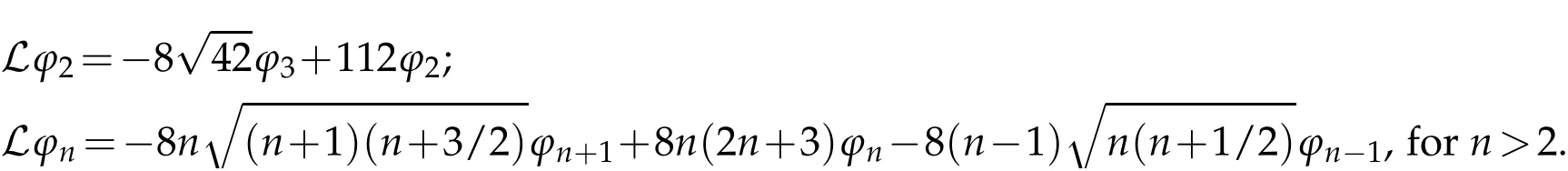
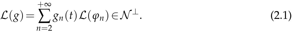
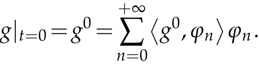
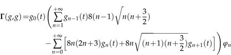
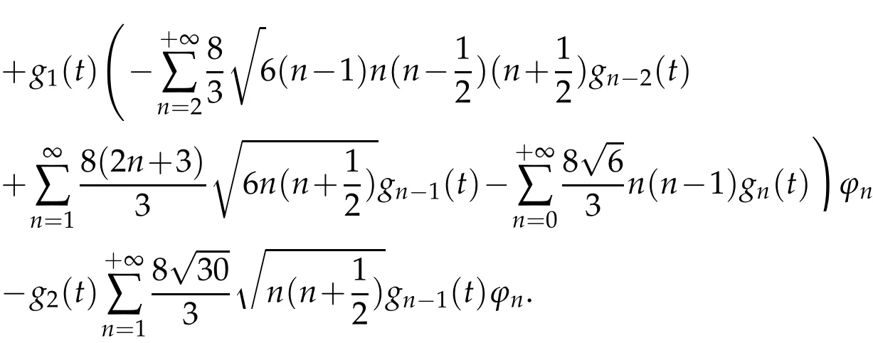
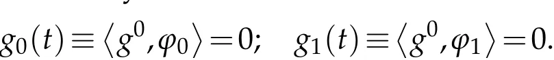
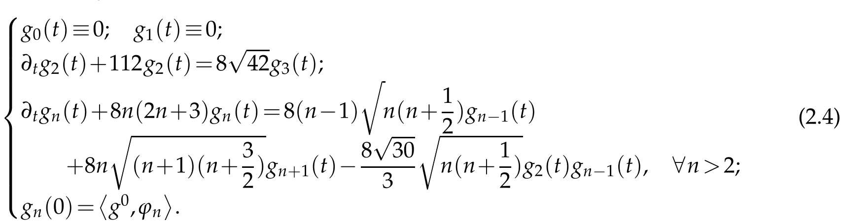
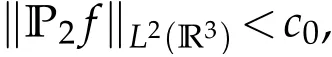
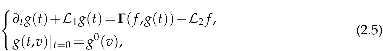
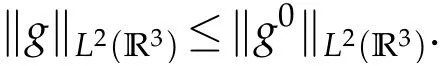
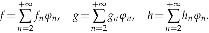
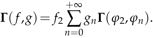
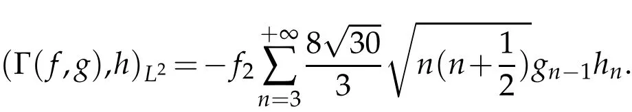
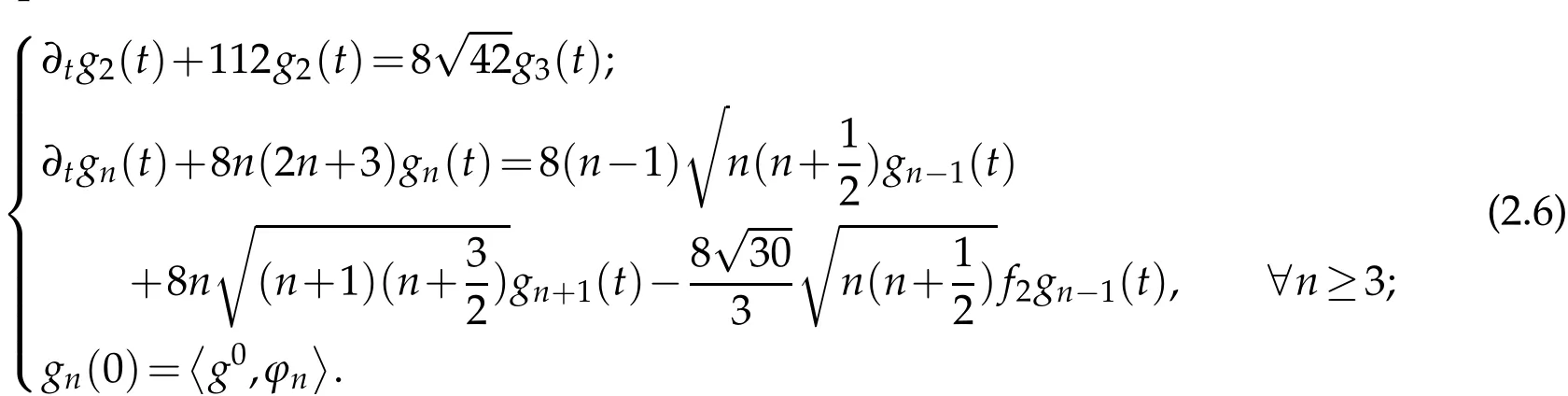
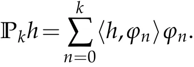
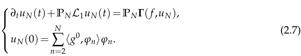
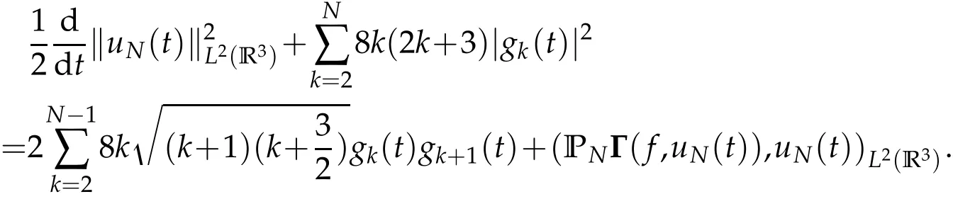
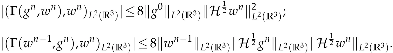
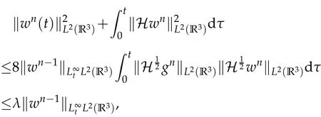
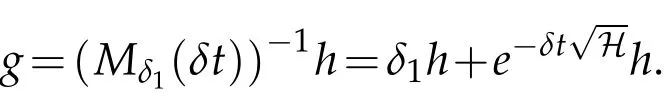
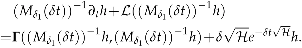
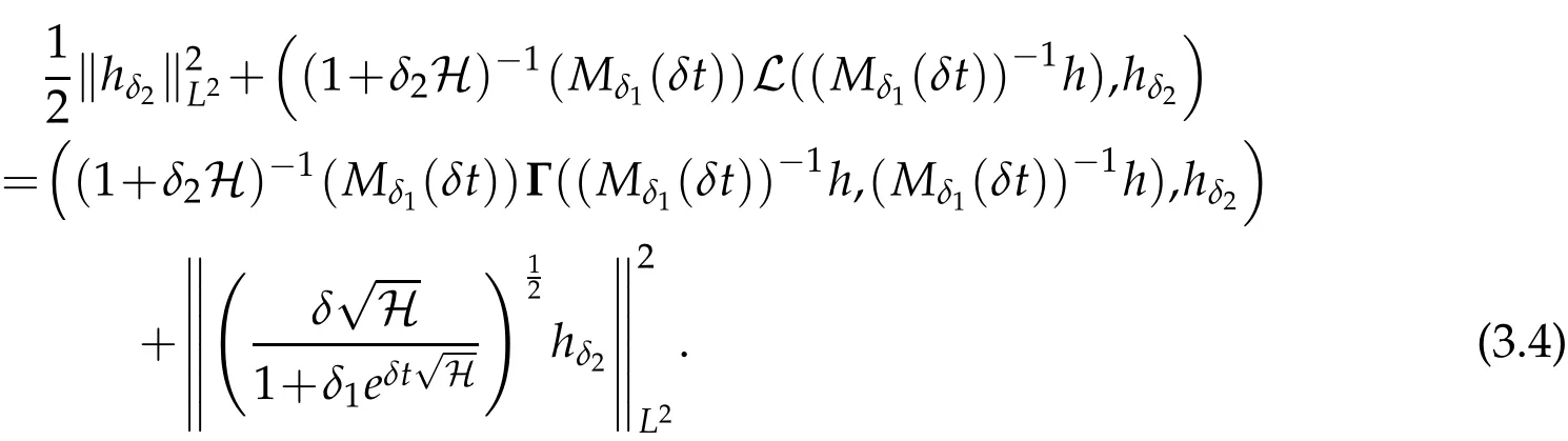
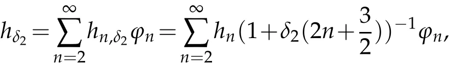
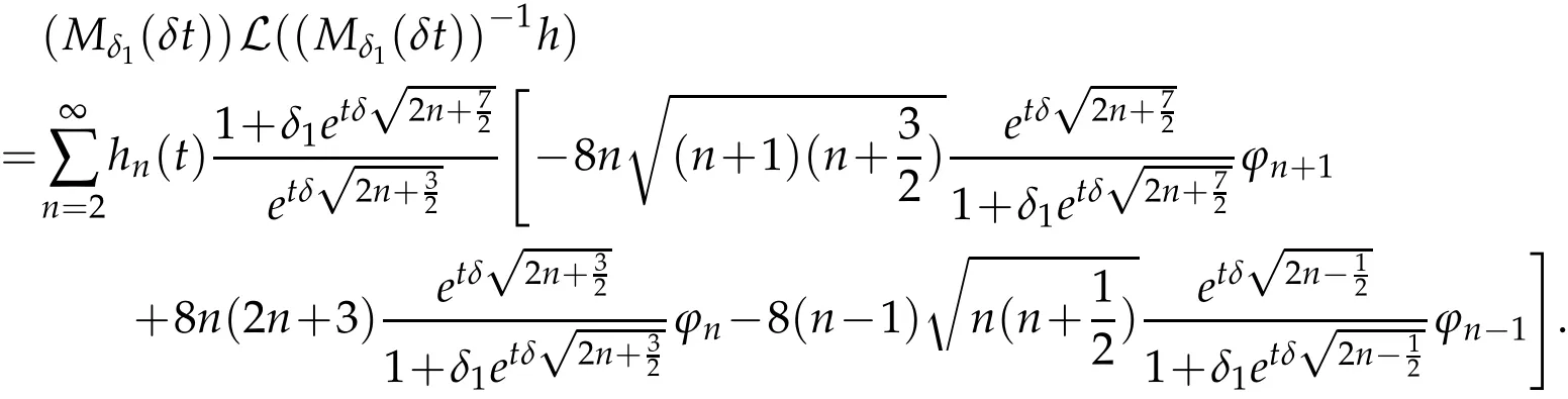
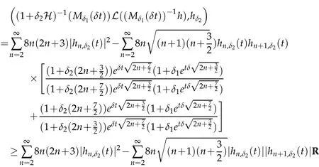
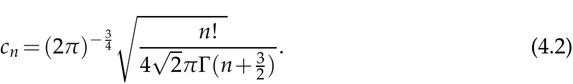
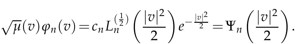
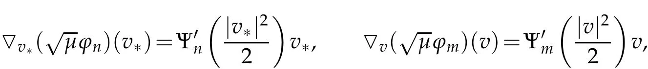
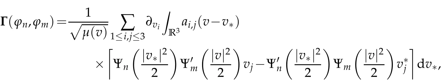
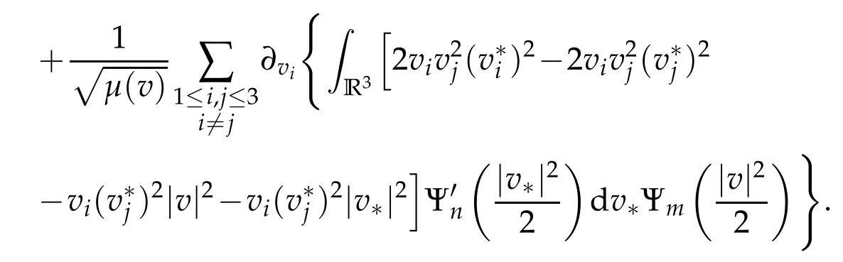
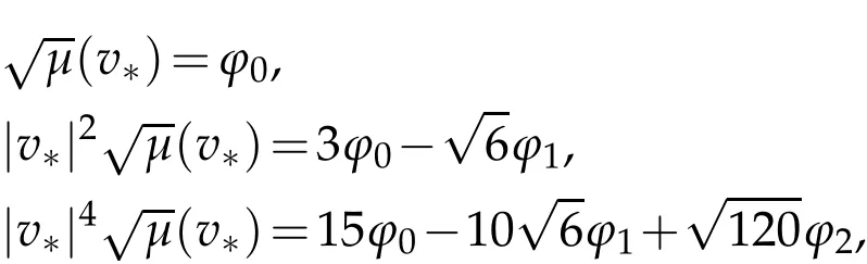
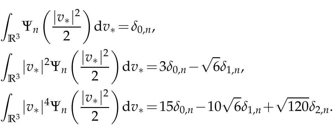
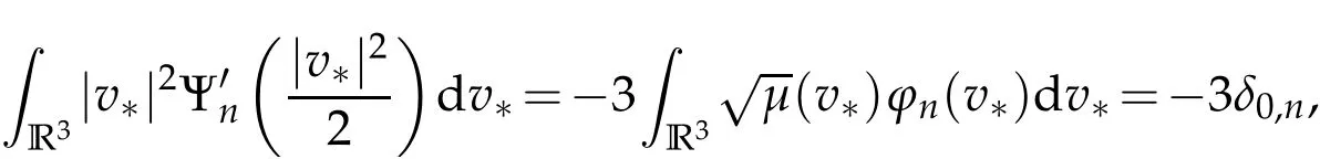
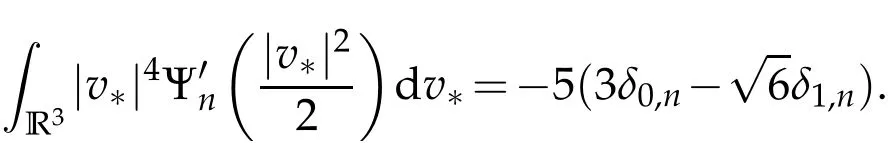
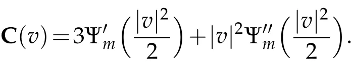
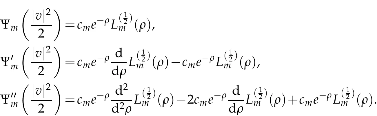
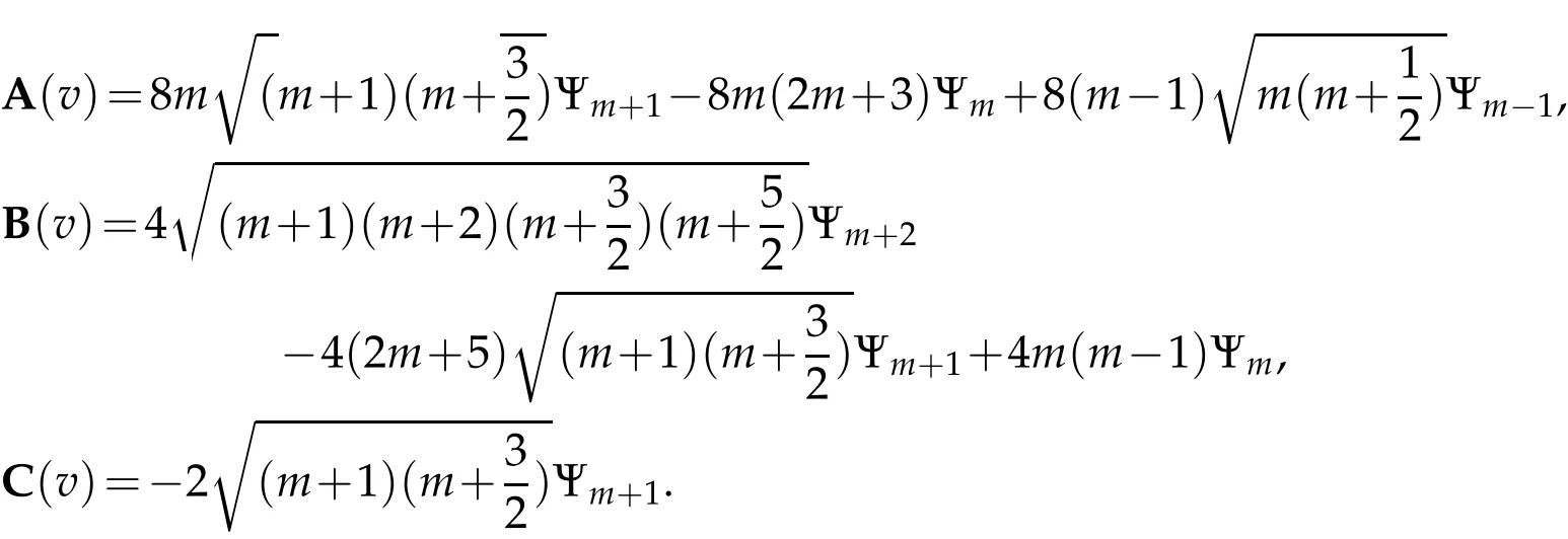
The projection function P:S′(R3)→N is well defined. The assumption of the initial datumf0in(1.1),transforms to beg0∈N⊥.We introduce the symmetric Gelfand-Shilov spaces,for 0 For more details,see in[3,Theorem 2.1]or in[4,Proposition 2.1]. The existence and regularity of the solution to Cauchy problem for the spatially homogeneous Landau equation with hard potentials has already been treated in[5,6]. We can also refer to[7,8]for the Gevrey regularity and Analytic smoothing effect for the solution of the Landau equation with hard potential.However,the mathematical technique in these works are mostly the energy methods. In this method,the smoothness effect of the Landau equation are almost not better than analytic smoothing effect. In 2012, Lerner, Morimoto, Pravda-Starov, Xu(LMPX) began to study the radially symmetric spatially homogeneous non-cutoff Boltzmann equation with Maxwellian mole cules by using spectrum analysis and then showed that the solution enjoys the Gelfand-Shilov smoothing effect in[9,10]and[11]. For Landau equation,Villani in[2]constructed a linear equation for the homogeneous Landau equation and MPX in[12]proved that the solution enjoys a Gelfand-Shilov regularizing effect in the class(R3). Recently, Li and Xu in[13]showed that global existence and Gelfand-Shilov regularizing properties of the solution to the Cauchy problem(1.2)for homogeneous non-cutoff Landau equation in Maxwellian molecules. From now on,the Gelfand-Shilov smoothing effect have never been studied in the non-Maxwellian case. In this paper,based on the spectral decomposition for the linear and nonlinear radially symmetric homogeneous non-cutoff Landau operators under the the hard potentialγ=2 in perturbation framework,we show the existence and the Gelfand-Shilov smoothing effcet for the solution to the Cauchy problem for this spatially homogeneous Landau equation. The main theorem is given in the following. Theorem 1.1.There exists a small positive constant ∈0>0, such that for any initial datum g0∈L2(R3)∩N⊥with the Cauchy problem(1.2)for radially symmetric homogeneous non-cutoff Landau equation in hard potential γ=2admits a global radially symmetric weak solution Moreover,we have the Gelfand-Shilov S11(R3)smoothing effect of Cauchy problem,for any given T>0,there exists a positive constant δ>0such that for all0≤t≤T, Remark 1.1.(1)The decompositions of the linear and nonlinear Landau operators under the hard potentialγ=2 are the technical part in this paper,in fact, the algebra structure of the linear Landau operator L is different from the Maxwellian molecules in[2]or[13]. (2)We think the regularizing property in the hard potentialγ=2 is similar to that in Maxwellian molecules. This work is a first step to study the Gelfand-Shilov smoothing effect for Landau equation in non-Maxwellian case.It is interesting to study more general case rather than the case ofγ=2. The rest of the paper is arranged as follows: in Section 2, we introduce the spectral analysis of the linear and nonlinear Landau operators, and the formal solution of the Cauchy problem (1.2) by transforming the linearized Landau equation into an infinite system of ordinary differential equations, then we construct the solution to the Cauchy problem for linear Landau equation. In Section 3, we prove the main Theorem 1.1. The spectrum analysis of the linear and nonlinear Landau operator is the technique part,which will be presented in Section 4. Diagonalization of the linear operators.We recall that{ϕn}constitute an orthonormal basis of(R3),the radially symmetric function space(see[11])with where Γ(·)is the standard Gamma function,for anyx>0, and the Laguerre polynomialof orderα,degreenread, In particular, Furthermore,we have,for suitable radially symmetric functiong, It follows that Triangular effect of the linear and non-linear operators.We study now the algebra property of the nonlinear operators Γ(ϕn,ϕm),and then the linear operator Similar to the proof of[11, Lemma 3.3], we can prove the following triangular effect for the nonlinear Landau operators on the basis{ϕn}in hard potentialγ=2. Proposition 2.1.LetΓbe the nonlinear Landau operator, the following algebraic identities hold true, where for convenience,we always set ϕ−1≡0. This proposition play a crucial role in the proof of the global existence of the solutions to the Landau equation under the hard potentialγ=2. We will give the proof of this proposition in the Section 4. Remark 2.1.Obviously,we can deduce from Proposition 2.1 that,forn∈N withϕ−1=0 and Then which satisfies that Lϕ0=Lϕ1≡0. Let P be the orthogonal Projection on N. Moreover,we have Then for radial symmetric functiong,one can verify that Now we solve explicitly the Cauchy problem (1.2) associated to the non-cutoff radial symmetric spatially homogeneous Landau equation with hard potentialγ=2 for the initial radial datag0∈L2(R3)∩N⊥. We search a radial solution to the Cauchy problem(1.2)in the form with initial data Remark thatg0∈L2(R3)∩N⊥is equivalent tog0radial and For suitable radially symmetric functiong,we have It follows from Proposition 2.1 that, For radially symmetric functiong,we can deduce from(2.1)in Remark 2.1 that Formally, we take inner product withϕnon both sides of the Cauchy problem(1.2), we find that the functions {gn(t)} satisfy the following infinite system of the differential equations Sinceg0∈N⊥,then it is obviously that The nonlinear Landau term turns out to be Furthermore,forn≥2, The infinite system of the differential equations(2.2)reduces to be Now we prove the existence of weak solution to Cauchy problem of the following linear Landau equation. Proposition 2.2.For any f,g0∈L2(R3)∩N⊥,there exists c0>0,such that f satifies whereP2f=f2ϕ2,then the Cauchy problem admits a weak solution Moreover,we have Before the proof of Proposition 2.2, we provide the sharp trilinear estimates for the radially symmetric nonlinear landau operator in the following Lemma. Lemma 2.1.For all f,g,h∈Sr(R3)∩N⊥,we have Proof.Letf,g,h∈Sr(R3)∩N⊥be some radially symmetric Schwartz functions, we can decompose these functions into the Hermite basis(ϕn)n≥0as follows It follows from Proposition 2.1 that, This implies that, By using the Cauchy-Schwartz inequality,one can verify that This ends the proof of Lemma 2.1. Now we are prepared to prove the Proposition 2.2. The proof of the Proposition 2.2.We search a radially symmetric solution to the Cauchy problem(2.5)in the form with initial dataRemark thatg0∈L2(R3)∩N⊥is equivalent tog0radial and Sincef∈L2(R3)∩N⊥, for radially symmetric functiong∈Sr(R3)∩N⊥, it follows from Proposition 2.1 that, Moreover,for thisg∈Sr(R3)∩N⊥,we can deduce from Remark 2.1 that withϕ−1=0 and Formally,we take inner product with{ϕn}n≥2on both sides of the Cauchy problem(2.5),we find that the functions{gn(t)}n≥2satisfy the following infinite system of the differential equations Let us now fix some positive integerN≥2 and define the following functionuN:[0,+∞[×R3→S′(R3)by wheregn(t) is the solution to the ODEs (2.6) forn≤N. Forh∈S′(R3), we defined thek+1 projection Pkthat Then forN≥2,PNuN=uNanduNsatisfies ForN≥2,taking the inner product ofuN(t)inL2(R3)on both sides of(2.7),we have Then one can verify from(2.6)that By using Cauchy-Schwartz inequality,we have We can conclude from Lemma 2.1 that By the assumption that‖P2f‖L2(R3) For anyN≥2,there exists positive constantC>0,we have also So that Eq. (2.7) implies that the sequenceis uniformly bounded in S′(R3)with respect toN∈N andt∈[0,+∞[. The Arzel`a-Ascoli Theorem implies that, there exists a subsequence{uNk(t)}⊂{uN(t)}such that Moreover,we have This shows that g(t)is a weak solution of Cauchy problem(2.5). We end the proof of Proposition 2.2. We recall the definition of weak solution of(1.2): Definition 3.1.Let g0∈S′(R3), g(t,v)is called a weak solution of the Cauchy problem(1.2)if it satisfies the following conditions: for any φ(t)∈C1([0,+∞[;S(R3)). Now we are prepared to prove Theorem 1.1. Existence.By using Proposition 2.2, we begin to prove the Global existence of solutions to the nonlinear Landau equation. For linear Landau equation (2.5), we consider the following sequence of iterating approximate solutions:starting fromg0(t,v)≡g0(v).Takingg=gn+1,f=gnin Proposition 2.2 gives,for anyt>0,there exists a constantδ0>0, Then it remains to prove the convergence of the sequence Setwn=gn+1−gn,one can verify from(3.1)that withwn|t=0=0. Sincewn∈N⊥,we have By the similar computation as(2.8),we get By using Lemma 2.1 again,we have For anyt≥0,,we obtain that, for some 0<λ<1. Then it follows that for some 0<λ<1. It concludes that{gn}is a Cauchy sequence which satisfies And its limit functiongis a desired solution to the Cauchy problem (1.2) int∈[0,+∞[.We obtain the global solution Gelfand-Shilov smoothing effect.Let 0≤δ,δ1≤1. Define The functionhdepends onδ,δ1.We can also write that The equation(1.2) reads as It follows that We define Then by multiplying(1+δ2H)−2hon both sides of(3.3),we have It follows from the Cauchy-Schwartz inequality that where Direct calculation shows that,for any 0 Then it follows from the Cauchy-Schwartz inequality that Remind thath∈N⊥,we can deduce from Proposition 2.1 that Since recall thatδ1,δ2≤1,we have Substituting the estimates(3.5)and(3.6)into(3.4),one can verify that We consider the fact that, then for 0 Therefore,choose∈,δsmall,we have This means that,for any 0 Letδ2→0,we have This ends the proof of Theorem 1.1. In this section, we will prove the proposition 2.1. This Proposition shows the spectral decomposition for the linear and nonlinear radially symmetric spatially homogeneous Landau operators under the hard potentialγ=2 in details. At the beginning, we introduce the kronecker function Proposition 4.1.LetΓbe the nonlinear Landau operator, the following algebraic identities hold true,for n,m∈N Proof.In all the proof of this proposition,we will set Ψk:R→R with Therefore,recalled from the definition ofϕn(v)that,forv∈R3, It follows that,form,n∈N where we used the notation Ψk(ρ)in(4.1)andfork∈N. Then where we have writtenv=(v1,v2,v3),v*=(v*1,v*2,v*3)∈R3and Direct computation shows that By using the elementary equalities Similar to the above symmetric property,and integration by parts,we can also prove that and By using the symmetric of the coordinate axis,we end the proof of Prop. 4.1. Now we prepare to prove the Proposition 2.1. The proof of Proposition 2.1.Denote that Recall from the definition ofin(4.1)and take intermediate variablewe have Using the formulas(141),(7),(12)of Chapter IV in[14]that,we have Substituting back to Proposition 4.1,we end the proof of Proposition 2.1. Acknowledgement The authors would like to express their sincere thanks to Prof. Chao-Jiang Xu for his stimulating suggestions.This research is supported by the Fundamental Research Funds for the Central Universities of China, South-Central University for Nationalities (No.CZT20007)and the Natural Science Foundation of China(No. 11701578).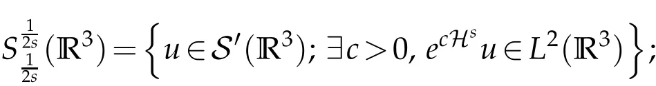


2 Spectral analysis and linear Landau equation
2.1 Spectral analysis


2.2 The Cauchy problem of linear Landau equation


3 The Proof of Theorem 1.1


4 The proof of Proposition 2.1


 Journal of Partial Differential Equations2022年1期