Ocean tide loading correction for InSAR measurements:Comparison of different ocean tide models

Zhou Wu ,Mi Jing ,Ruy Xio ,Jing Xu

a School of Earth Science and Engineering,Hohai University,Nanjing,211100,Jiangsu,China

b School of Geospatial Engineering and Science,Sun Yat-Sen University,Guangzhou,510275,China

Keywords:InSAR Large-scale InSAR Ocean tide loading Ocean tide models

ABSTRACT With the rapid development of modern Interferometric Synthetic Aperture Radar (InSAR)missions,SAR instruments with wider coverage can be used to monitor the ground surface deformation from regional to global scale.However,the ocean tide loading (OTL) displacement is becoming a primary source of errors.It contributes to a long-wavelength signal in InSAR interferograms,leading to errors from millimeter to centimeter-level in InSAR deformation monitoring,especially over coastal areas.Although the state-of-the-art has applied ocean tide models to mitigate the errors,the difference between them and their impact on InSAR measurements are rarely discussed.In this paper,we compare representative ocean tide models and investigate their effects in the correction of OTL errors.We found that (i) the modeled OTL displacements from different models show little difference over interiors far from the ocean,while disagreement becomes larger over coastal areas;(ii)the magnitude of OTL artifacts may be greater than the atmospheric delays in some coastal areas,and the correction using ocean tide models can effectively attenuate the OTL effects for large-scale InSAR measurements;(iii) when correcting the OTL errors for InSAR measurements,the global model TPXO and FES are recommended because of their better overall performance,while the NAO model performs the worst.The local models with high spatial resolution can help improve the capability of coarse global models in complex topographic areas.

1.Introduction

Interferometric Synthetic Aperture Radar (InSAR) is a powerful geodetic technique capable of measuring land surface deformation[1].With the successful launch of the European Space Agency's Sentinel-1 satellites,more and more studies focus on ground surface mapping at a larger scale,i.e.,territorial and national regions[2,3].In comparison with sources of error at a local scale,the correction for long-wavelength errors,such as tropospheric delays,ionospheric errors,and orbital errors,plays a more important role in large-scale InSAR processing.Generic Atmospheric Correction Online Service for InSAR (GACOS) [4],modeling with the external data(e.g.,network GPS data,MERIS and MODIS water vapor data),faraday rotation inversion [5],and polynomial fitting [6] has been widely applied in last decades to mitigate long-wavelength errors with different successes.

Recent studies show that the ocean tide loading (OTL)displacement can contribute to the longer-wavelength signal in interferograms and affect the large-scale InSAR detection in varying degrees.DiCaprio &Simons [7] first used the GOT00.2 ocean tide model to quantify the OTL displacement over the specific area,proving that OTL can cause millimeters to centimeters displacement near coastal regions.The conclusion demonstrates the necessity of OTL correction for areas with slow surface motion at a large scale.Lei et al.[8]compared the InSAR results with the Global Positioning System (GPS) results,concluding that the accuracy of InSAR measurement can increase by around 20%if OTL correction is considered.Peng et al.[9] used the bilinear ramp function to remove the orbit errors in the interferograms and found that the remaining long-wavelength signal is mainly OTL displacement.Furthermore,they applied the kinematic precise point positioning(PPP)solution and the wavelet transform method to model the OTL displacements,respectively[10,11].It was proved that the accuracy of modeled OTL from geodetic techniques(i.e.,GPS and InSAR)can be comparable to ocean tide models.Yu et al.[12] established a global standard deviations(STD)map of OTL to show the activity of OTL globally.Considering that the InSAR technique uses the differential observation between two arbitrary acquisitions to map the surface change,the higher STD value implies larger OTL errors in InSAR interferograms.A few studies also analyzed the differences between various ocean tide models.For example,in Li et al.[13],the impact of two global models (GOT4.8,HAMTIDE11a) and a local model (OSU.CHINASEA.2010) were evaluated on coastal deformation mapping with InSAR measurements.Despite the great interest,many representative ocean tide models are not fully explored,and their impacts on the precision of large-scale InSAR deformation monitoring are unknown yet.

To better understand the effectiveness of global and local ocean tide models on InSAR measurements and further extend the InSAR technique towards large-scale applications,in this paper,we compare the differences between seven global ocean tide models and three local models over three characteristic coastal regions with great fluctuations of the tidal waves,then evaluate their performances on the Sentinel-1 dataset.

2.Study area and dataset

2.1.Study area

Previous studies have proved that the standard deviation of OTL displacement over the regions in Canada,Brazil,and France are relatively large [12].Three representative areas (Fig.1) distributed with different geographic conditions are therefore selected to test the OTL correction.Moreover,the great fluctuation of tidal waves and different types of coastline can help better to evaluate the performances of various ocean tide models.

The first study region Baffin Island is the biggest island located in Canada,surrounded by the Labrador Sea(Fig.1(a)).The irregular ocean depth and basins change the bulges,which cause the large tidal variations near the coastline [14].The southeast part of the island,with its tortuous coastline and many fjords,is one of the regions most affected by ocean tide loading effects in the world.The second region lies in tropical South America near the equator(Fig.1(b)).It is part of the Maranhao state in Brazil,and its southeastern coast faces the Atlantic Ocean.Reference [15] has shown that the oceanic tide close to the equator displays a high amplitude because of the intense movement of the Atlantic.The ocean tide loading has affected this area along the coastline for many years.Similarly,with the strong ocean tides on the Atlantic and Channel coasts,Europe,especially the UK,Ireland,and France,is often used as a study area for investigating the OTL displacement[16-18].We choose the Brittany Peninsula located on the northwest coast of France as the third region (Fig.1(c)).

2.2.SAR dataset

Six single-look complex(SLC)images,including ascending and descending orbits of Sentinel-1A/B with TOPS mode,are selected as shown in Table 1.The images with a relatively short temporal baseline are chosen to ensure very weak surface movement during the imaging period.In this sense,the dominant signals after phase filtering and unwrapping are long-wavelength errors,so that we can use STD to evaluate the noise level in interferograms before and after correction.All SLC SAR images were processed with GAMMA software,and we down-looked the interferograms resolution of 100 m.Precise Orbit Ephemerides(POE)file provided by European Space Agency was used to remove the orbital errors.The topography phase was removed using the TerraSAR-X add-on for Digital Elevation Measurements(TanDEM-X).We reduced stochastic noisefor each interferogram by means of the Goldstein filtering.An unwrapping algorithm based on minimum-cost-flow was then employed to unwrap each interferogram.

Table 1 SAR images dataset.

Fig.1.Overview of the study areas.(a)Baffin Island,northeast of Canada;(b)Brittany Peninsula,west of Paris;(c)Maranhao State,west of Brazil.Red boxes represent the coverage of SAR images.The yellow pentagrams represent the IGS stations.

3.Method

3.1.Estimation of OTL displacement

According to the Farrell loading theory [19],ocean tide loading can be modeled by a global integral:

where

L

（θ，λ，

t

）is the OTL (including tilt,strain,gravity,displacements,etc.) at an observation location (θ，λ) at a certain time

t

;The density of ocean ρ is the annual average value computed from the International Equation of State for seawater,combined with the ocean's temperature and salinity from 2009 World Ocean Atlas[20,21];

H

（θ，λ，

t

）is the tide height at load point (θ，λ) at the same time

t

.φ is the angular distance between the sites and the loading points,and

A

is the azimuth between the load point and the observation;

ds

denotes each pixel of the specific ocean tide model grid,and the integral is implemented on the whole pixels over the entire world's ocean grid;

G

is the mass-loading Green function including vertical and horizontal components.Applying the Lovenumbers

h

and

l

,the Green function for vertical displacements and horizontal displacements can be written as: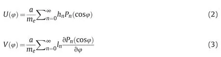

where

a

and

m

are radius and mass of the Earth,

P

is the Legendre function of spherical harmonic degree.The mass-load love numbers

h

and

l

are computed up to degree 10,000 using the numerical method with Kummer's transformation to accelerate the convergence,supplemented by the

n

=∞limit [19].To assess the capability of different ocean tide models,we fix the Earth model as PREM [22].The reference frame is based on the center of mass of the load and the Earth [23,24].Eq.(1) is based on one tide only,usually we consider eight principal tides (the semidiurnal M2,S2,K2,N2,and the diurnal K1,O1,P1,Q1).The total displacements can be expressed as: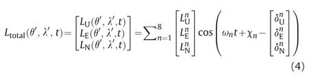

Due to the side-looking radar imaging geometry,the three direction displacements are projected into the LOS (line of satellite)direction by:

where θ is the incidence and α is the heading angle;The LOS displacement

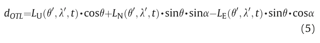
d

is converted to phase Φand then subtracted from the unwrapped phase.The procedure is shown in Fig.2.

3.2.Ocean tide models

According to Eq.(1),the most critical step to estimating OTL displacement is determining the tide height,which can be obtained from ocean tide models.Modern tide models are split into two categories.(i)Purely hydrodynamic models(non-data-assimilating models) without any data constraint;(ii) Hydrodynamic and empirical models with assimilating data.Purely hydrodynamic models calculate tides by imposing the respective forcing without data constraints.However,their accuracies are far less than those with altimetry data [25].Therefore,we focus on the second category.The hydrodynamic and empirical models have been vigorously developed since the launch of the altimetry satellites designed to measure tides height.The altimetry data(i.e.,T/P,ERS-1/2,Jason-1/2,TPN-J1N,GFO,and ENVISAT) together with tidal gauges are the main sources used as the constraints during data assimilation.Seven widespread global hydrodynamic and empirical models used in this paper include NAOglobal,GOT4.8,FES2014,DTU10,EOT11a,HAMTIDE11a,and TPXO9-atlas-v4,the details have been listed in Table 2.

In addition to the global model,we also consider the local models.There are 22 local models distributed worldwide,and each of them only covers a portion of the earth.According to the study regions,we choose three local models.The name and coverage of the three local models are listed in Table 3.All models starting initially with Osu are produced at Oregon State University by S.Y.Erofeeva and G.Egbert [33].Because the OTL displacement is computed through the convolution integral over all water areas globally(Eq.(1)),the local model cannot be used directly.Thus,it is necessary to combine with the global model to compensate for the low resolution of some global models in local areas.To this end,we used the GOT4.8 as a compliment due to its high accuracy in the deep ocean [25].We will investigate whether a local model with high spatial resolution can improve the capability of the global model in local areas.

Table 2 Participating global ocean tide models.

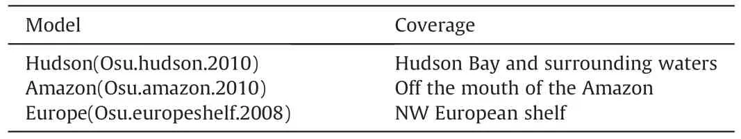
Table 3 Local models’names and regions[34].

4.Results and discussions

4.1.Comparison of ocean tide models

Section 2 shows various ocean tide models from the earlier NAOglobal to the latest TPXO9-atlas-v4,these models are separately input to the Some Programs for Ocean Tide Loading(SPOTL)software [35,36] to calculate the OTL displacement.To this end,a grid with a resolution of 0.0333was resampled based on the coverage of SAR images.Then 3D (east,north,and up) displacements were computed at each observation time according to each grid coordinate and projected into the LOS direction.To coregistrate the OTL displacement grid and unwrapped phase in SAR images,we further interpolated the grid from 0.0333to 0.0008333by the bilinear interpolation.Finally,a total of eight LOS OTL displacement maps were obtained,and each of them corresponds to an ocean tide model.To better show the differences between models,we differentiated each two LOS OTL displacements maps as shown in Figs.3-5,in which the scatter plots with respect to difference maps are counted in the lower triangular portion.

Fig.2.Flow chart of OTL correction for InSAR measurements.

In Fig.3,eight models are consistent well over most of the area until some areas near the narrow channels,where the NAO ocean tide model has the worst performance (see the first row and column in Fig.3 for details) since it has the largest dispersion up to 20 mm in comparison with others.In contrast with the NAO model,GOT model shows better agreement,although they share the same resolution of 0.5.We,therefore,may conclude the inconsistency between NAO and other models is the estimate accuracy rather than resolution.HAMTIDE,DTU,and EOT models have the same resolution of 0.125and fit each other comparably well,the maximum difference is less than 10 mm.Similar behavior can be observed in the Hudson,FES,and TPXO models with the higher resolution,which corresponds to 0.0333,0.0625,and 0.0333,respectively.The difference between them is less than 3 mm.This proves that the performance of FES and TPXO global models has been able to match the high-resolution local model over this region.It is worth noting that the models with the same low spatial resolution (HAM,DTU,and EOT) show large anomalous with those models with a high spatial resolution (Hudson,FES,and TPXO) in the near-channel zone.These suggest that the performance of models is also related to their spatial resolution.

Analogously,the inconsistency between NAO and other models becomes more significant in Brazil in Fig.4.The difference between them increases from～5 mm in the inland area to～14 mm near the north coast,and the maximum value exceeds 18 mm.In addition to the NAO,other models also show some differences in varying degrees.For example,the values of GOT model are a few millimeters large than the other models over most regions,implying that there exists an inherent constant bias between them.FES,TPXO,and the local Amazon model don't fit as well as they do in Canada,they show small anomalous in some parts of the coastal areas where the discrepancy up to 5 mm.

In Fig.5,the biases between all models vary within the interval between 0 and 3 mm except for those including the NAO model,showing the consistency for the seven models.The difference reaches about 5 mm when the NAO model is included,showing again the inconsistency of the NAO model in comparison with others.It is worth noting that the differences in OTL displacements are all large along the coast and decrease with distance away from the coastline.This is due to the fact that coastal regions are closer to the mass load point and,therefore,more sensitive to loading displacement.

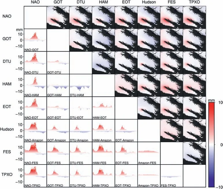
Fig.3.Differential displacement maps estimated from various ocean tide models,and corresponding scatter plots in Canada.

4.2.InSAR OTL correction

From the cross validation in the previous section,we found that the NAO model has a larger error than others by modeling OTL displacements.To further assess their performance on OTL correction for InSAR measurements,we remove the OTL displacement from unwrapped interferograms,and use STD to evaluate the overall noise level of the interferograms before and after OTL correction.For the sake of the validation with the precise GPS solution,we also remove the atmospheric delay and solid body tide by the Generic Atmospheric Correction Online Service [4] and Solid program(https://geodesyworld.github.io/SOFTS/solid.htm) respectively.As shown in Figs.6-8,significant long-wavelength signals can be clearly observed in all original interferograms over three areas,even if the atmosphere and solid body tide are corrected.The magnitude decreases gradually from the coastal area to the inland area.We modeled the OTL displacement according to the coverage of interferograms,from which we can see that the characteristics of the ramp are very similar to those of OTL displacements.Quantitatively,STD values drop by 51%,17%,and 38% in comparison with original ones in Canada,Brazil,and France,respectively.Furthermore,the differences of STD among all models after correction are quite small and close to the sub-millimeter level.The maximum difference values are 0.5 mm,0.5 mm,and 0.2 mm in Canada,Brazil,and France,respectively.Therefore,we may conclude that different ocean models have little difference on the correction of InSAR measurements,even for the STD values of the interferograms corrected from the NAO model which has the maximum dispersion generally.Moreover,along the profiles it is clear that the points show large discrepancies with the range from millimeter to centimeter in coastal areas.As the points get further from the coastline,the differences become smaller,similar to the analysis in section 4.1.Because these models give rise to the difference only over local regions along the coast,the STD value may underestimate the effect of models.We therefore further validate the results with the external GPS data from the stations close to the coastline.

We chose three IGS stations located in Iqal,Salu,and Brst,respectively(Fig.1).The necessary files,including observation files,precise orbits,clock products,are provided by Crustal Dynamics Data Information System (CDDIS).These files are processed by PPPH software [37] in static PPP mode into daily solution.After converting 3D displacements into the LOS direction,the displacement calculated by PPP,together with LOS displacements estimated from InSAR after OTL correction under different models,are listed in Table 4.Due to the shorter visiting period of the Copernicus Programme satellite constellation,the displacement at these locations should be close to zero,which has been validated from the PPP solution.However,the deformation estimated from InSAR measurement is far from zero as the long-wavelength errors,such as tropospheric delays,solid earth tides,ocean tide loading,dominate the interferometric signals.When correcting the tropospheric delays and solid body tide displacement,the InSAR measurements are closer to the GPS-PPP solutions,with the accuracy improved by 9%,47%,and 41% in Iqal,Salu,and Brst,respectively.After Applying the OTL corrections,the accuracy is improved by about 69%,15%,and 49%.This demonstrates that OTL-induced surface displacement palys a primary role in InSAR errors in comparison with tropospheric delays and solid body tide over these local coastal areas.

Fig.4.Differential displacement maps estimated from various ocean tide models,and corresponding scatter plots in Brazil.

Fig.5.Differential displacement maps estimated from various ocean tide models,and corresponding scatter plots in France.

Fig.6.Original interferograms,GACOS,and Solid corrected interferograms,modeled OTL displacement maps(row 1)and GACOS,Solid,OTL corrected interferograms(row 2)with their standard deviation over Baffin Island in Canada (top).Change of pixel values from A to B and C to D (bottom).The O-G-S indicates Original-GACOS-Solid.

Fig.7.Original interferograms,GACOS and Solid corrected interferograms,modeled OTL displacement maps (row 1)and GACOS,Solid,OTL corrected interferograms (row 2)with their standard deviation over Maranhao state in Brazil.(top).Change of pixel values from A to B and C to D (bottom).The O-G-S indicates Original-GACOS-Solid.

In Table 4,it is observed that the better-performing models are TPXO and FES,by which the corrected InSAR measurements are closest to the GPS-PPP solution at the Salu site.In Iqal and Brst,they perform similarly or marginally better than the others.The local model (e.g.,refined GOT model) is better than GOT model in Iqal,but worse at Salu and Brst.This indicates that the high-resolution local model can help improve the capability of the coarse global model over rough topography.As for the areas without complex coastlines,the global model is already quite accurate,even for models of coarse spatial resolution like GOT.

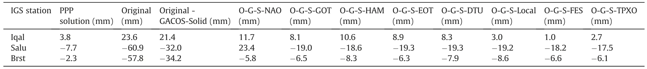
Table 4 IGS station displacements obtained by InSAR and PPP.The O-G-S indicates Original-GACOS-Solid.

Fig.8.Original interferograms,GACOS and Solid corrected interferograms,modeled OTL displacement maps (row 1) and GACOS,Solid,OTL corrected interferograms(row 2)with their standard deviation over Brittany Peninsula in France.(top).Change of pixel values from A to B and C to D (bottom).The O-G-S indicates Original-GACOS-Solid.

The NAO model has the worst accuracy in total,although it performs best at the Brst site.Recall the results in Figs.3 and 4,the NAO model has shown an opposite tendency,i.e.,larger than others in Canada and smaller in Brazil.This phenomenon is consistent with the comparison in Table 4,in which we can see that the NAO model also shows the same opposite tendency at the two sites.Therefore,we can infer that the NAO model has some kinds of systematic bias in the Canada and Brazil regions and is not suitable as a corrected model.The reason behind is that the NAO model does not predict the tidal height accurately enough and this error is propagated to the tidal loading displacement.

5.Conclusion

The effect of ocean tide loading is a main error source in largescale InSAR monitoring over the coastal areas and should be carefully evaluated by ocean tide models.However,the knowledge on the differences between ocean tide models and on the optimal selection for mitigating the OTL effects in InSAR measurement is not clear yet.To solve the issues and further extend the standard InSAR technique towards the large-scale processing with high accuracy,we present a review of the widely used ocean tide models and conduct a comparison analysis among them.The performances of seven global and three local models on Sentinel-1 dataset are evaluated over three regions characterized by the great fluctuation of tidal waves.It comes to the following conclusions:

• The OTL displacement maps derived from various ocean tide models agree well over inland areas far from the coast.The discrepancy mainly appears in coastal areas with complex topography,such as those in Canada and Brazil,where the differences between models are within 5 mm over the inland regions.However,they increase rapidly to the centimeter level when closer to the coastline.The results demonstrate that it is necessary to select a suitable model near the coastal areas,and the impact of models on inland regions can be generally neglected.

• The OTL can introduce long-wavelength noises whose magnitude may be even greater than atmospheric delays.This kind of non-tectonic signal needs to be corrected carefully to improve the degree of confidence when interpreting large-scale ground motions.In this paper,we use standard deviation and external GPS data to evaluate the performance of ocean tide models and found that the model-corrected method is effective in weakening the effects of the OTL,and the accuracy of InSAR measurements can be enhanced by up to 69%.

• The global model TPXO and FES are recommended because their overall performances are slightly better than others in the three study areas,whereas the NAO model is not suggested in general.For coastal areas with complex topography,the local model can help to improve the capabilities of coarse global models to some extent.

Conflicts of interest

The authors declare that there is no conflicts of interest.

Acknowledgments

This work was supported by the Natural Science Foundation of China (grant Nos.42074008,41804005,42174018).

The authors would like to thank Dr.Duncan Agnew for the SPOTL software,Dr.Dennis Milbert for Solid program.We acknowledge the European Space Agency for providing the Copernicus Sentinel-1 SAR data,and the e GACOS website (http://ceg-research.ncl.ac.uk/v2/gacos/) for GACOS products used.Finally,we thank the reviewers and editors for their very helpful comments and suggestions.