Spatial diff erence in net growth rate of Yesso scallop Patinopecten yessoensis revealed by an aquaculture ecosystem model*

Xueliang NAN, Hao WEI, Haiyan ZHANG, Hongtao NIE

School of Marine Science and Technology, Tianjin University, Tianjin 300072, China

Abstract Identifying the main factors on spatial diff erences in net growth rate of Yesso scallop ( Patinopecten yessoensis) in culture system is the key to eff ective aquaculture management and development. Coupling a 3D ecosystem model (ROMS-CoSiNE) with a dynamic energy budget model for scallops, a Yesso scallop culture ecosystem (YeSCE) model was established with which scallop growth was simulated with real seeding density and juvenile size from local aquaculture experiments from December 1, 2012 to November 30, 2013. Results show that the YeSCE model has reasonably simulated the environmental variation and scallop net growth rate in the Changhai sea area. The growth of scallops was slow in winter and midsummer and was limited mainly by temperature. Food availability was a key factor that contributed to the fast growth of the scallops during spring to early summer and in autumn. Generally, the scallops cultured in the north part of the Changhai sea area grew faster than those in the south; and the net growth rate for scallops cultured near the island was signif icantly higher compare to the others, which is probably correlated to the spatial distribution of food availability. Based on the correlation analysis, the spatial diff erences of the net growth rate were largely aff ected by the length of the match timing of temperatures and food availability.The results of this study provide a scientif ic support for optimizing bottom culture planning and adjusting bottom culture methods.

Keyword: 3D ecosystem model; shellf ish aquaculture; Yesso scallop; Patinopecten yessoensis; net growth rate; Changhai sea area

1 INTRODUCTION

China has recorded higher annual aquaculture production than the rest of the world combined since 1991 (FAO, 2020). In 2018, mariculture production in China exceeded 20.31 million tons, accounting for 66% of the global mariculture production (Fishery Administration Bureau of Ministry of Agriculture and Rural Areas et al., 2019; FAO, 2020). For the sustainable development of aquaculture, the strategic choice of China is to accelerate the green development of aquaculture in the new era (Chen, 2019). It is our duty to promote the green development of aquaculture and to accelerate actively the transformation of developing mode in aquaculture (Chen, 2019).Scientif ic planning and management of culture areas are one of the signif icant methods to realize green development, which is based on the research on the spatial diff erence in the net growth rate of cultured organisms.

Yesso scallop is one of the widely cultured economic shellf ish species in China (Zhao et al.,2019). Changhai sea area is now the largest Yesso scallop culture area in the North Yellow Sea, including bottom and raft culture (Yuan et al., 2010; Li et al.,2012). In addition to natural predators, the growth of cultured scallops can be aff ected by overcapacity,rapid temperature changes, and food shortages (Rico-Villa et al., 2009; Jiang et al., 2018; Zhao et al., 2019),resulting in an uneven spatial distribution of harvestable biomass in the areas (Liu et al., 2014;Zhao et al., 2019). The Changhai sea area was aff ected by the northern Yellow Sea cold water mass, the Yellow Sea warm current, tidal fronts, etc. (Guan,1963; Chen, 2009; Nan et al., 2020), and it encompasses a rich array of physical and biological processes. The impact of the spatial diff erence of environmental dynamics on the bottom cultured Yesso scallop needs scientif ic evaluation. Several studies conducted f ield surveys to research the Yesso scallop growth in some sites in the study area (Jiang,2013; Zhang et al., 2017; Jiang et al., 2020). However,the research on the net growth rate in most areas is not enough, which aff ects the scientif ic planning and management of the aquaculture area. Therefore, it is necessary to simulate and analyze the key factors inf luencing scallop growth in diff erent areas and diff erent periods after one year of uniform seeding of scallop culture and f ind out the reason for the inf luence on spatial diff erences in the net growth rate.

The individual growth model based on the dynamic energy budget (DEB) theory (Kooijman, 2010),named the DEB model, is a widely used model of methodology for quantifying individual shellf ish growth. The theory has been applied to a variety of shellf ish species based on observed temperature and food availability (Pouvreau et al., 2006; van der Veer et al., 2006; van der Meer and Kooijman, 2014;Lavaud et al., 2017; Stavrakidis-Zachou et al., 2019;Jiang et al., 2020). However, due to the sporadic observation in space or time under most circumstances,it is hard to copy the temperature and food availability of the culture. Thus, the uncertainty may be large in the modeled results. The latest development in this f ield involves coupling the DEB model with a 2D physical-biogeochemical model (Guyondet et al.,2010; Filgueira et al., 2014) or a 3D hydrodynamic model and box model of food at the bottom boundary layer (Zhao et al., 2019). However, water temperature and food availability in the North Yellow Sea is largely controlled by the hydrodynamic and thermal conditions, including the circulation, solar radiation,seasonal stratif ication, freshwater discharge, among others. Using the bottom box model alone cannot replace the dynamic changes of food availability in the natural condition. Therefore, our research team built a physical-biological coupling model. The model is based on a 3D high-resolution, regional circulation model conf igured with the Regional Ocean Modeling System (ROMS) (Shchepetkin and McWilliams,2005) and an ecological model called the CoSiNE(carbon, silicate, and nitrogen ecosystem) model (Xiu and Chai, 2014). All the components of ROMSCoSiNE are aff ected by physical processes, such as advection and diff usion (Zhou et al., 2017). ROMSCoSiNE model provided more detailed 3D data of temperature and food availability, which serves as the forcing conditions to the DEB model to enhance our estimation on the net growth rate of Yesso scallop.

The objective of this study is to develop a Yesso scallop culture ecosystem (YeSCE) model considering physical-biological condition and individual growth of Yesso scallop to guide the aquaculture in the Changhai sea area and possibly the other places in the future, to predict the areas with little-to-no data, and determine the inf luence factors of spatial diff erence in net growth rate of scallops.

2 MATERIAL AND METHOD

2.1 Study area and f ield data

Changhai sea area is located in the North Yellow Sea to the east of Liaodong Peninsula (Fig.1a, red box). The area is aff ected by the Yellow Sea Warm Current in winter and the North Yellow Sea Cold Water Mass in summer (Guan, 1963; Chen, 2009).The main study area for YeSCE model includes the aquaculture area of Zhangzi Island, Changshan Islands, and Haiyang Island (Fig.1b). Traditional raft culture (blue polygon) and bottom culture areas(yellow polygon) are shown in Fig.1b (Yuan et al.,2010; Li et al., 2012). In this study, it is assumed that the whole sea area was bottom-cultured, and the results can be used as a basis for future planning.

The colormap represents the water depth in Fig.1a,and the black dots represent the survey stations of the National Nature Science Foundation of China (NSFC)Ship-time Sharing Project in the North Yellow Sea.The conductivity-temperature-depth data measured with a f luorometer (CTD; RBR 620) from September 10 to 12, 2017, the vertical temperature prof iles at every transect station with a sampling rate of 6 Hz.The temperature and chlorophyllafrom the bottom layer were measured by SBE 911 on July 9-11, 2016.Station ZZD (red triangle in Fig.1b) includes a bottom-mooring frame that carries an upward-facing acoustic Doppler current prof iler (ADCP, RDI 300K)and a CTD (RBR 420), which collects temperature and current data near the bottom layer from July 10 to August 26, 2017, the sampling frequency of 15 s (Nan et al., 2020). The temperature and chlorophyll-adatawere daily averaged for the following analysis. The survey stations for scallop growth are shown in red stars in Fig.1b. Shell length and f lesh dry weight were recorded in station ZZD_01 from December 2012 to November 2014 (Jiang et al., 2020), with which the half-saturation coeffi cient was calibrated; and temperature and chlorophyllawere recorded daily(Jiang et al., 2020). Shell lengths were recorded in stations ZZD_02 and ZZD_03 from December 2012 to August 2013 (Jiang, 2013), with which the scallop growth was determined. Temperature and chlorophyllawere monthly measured at 2-m depth in station ZZD_04 from January to December 2007 (Yuan et al.,2010). In addition, three representative sites (red squares in Fig.1b) S1(16 nautical miles south of Zhangzi Island), S2(near Zhangzi Island), and S3(16 nautical miles north of Zhangzi Island and the location the same to station ZZD_04) (Fig.1b) selected in latitudinal direction were used to analyze the spatial and temporal diff erences of the relationship among temperature, food supply, and scallop growth in section Discussion later.

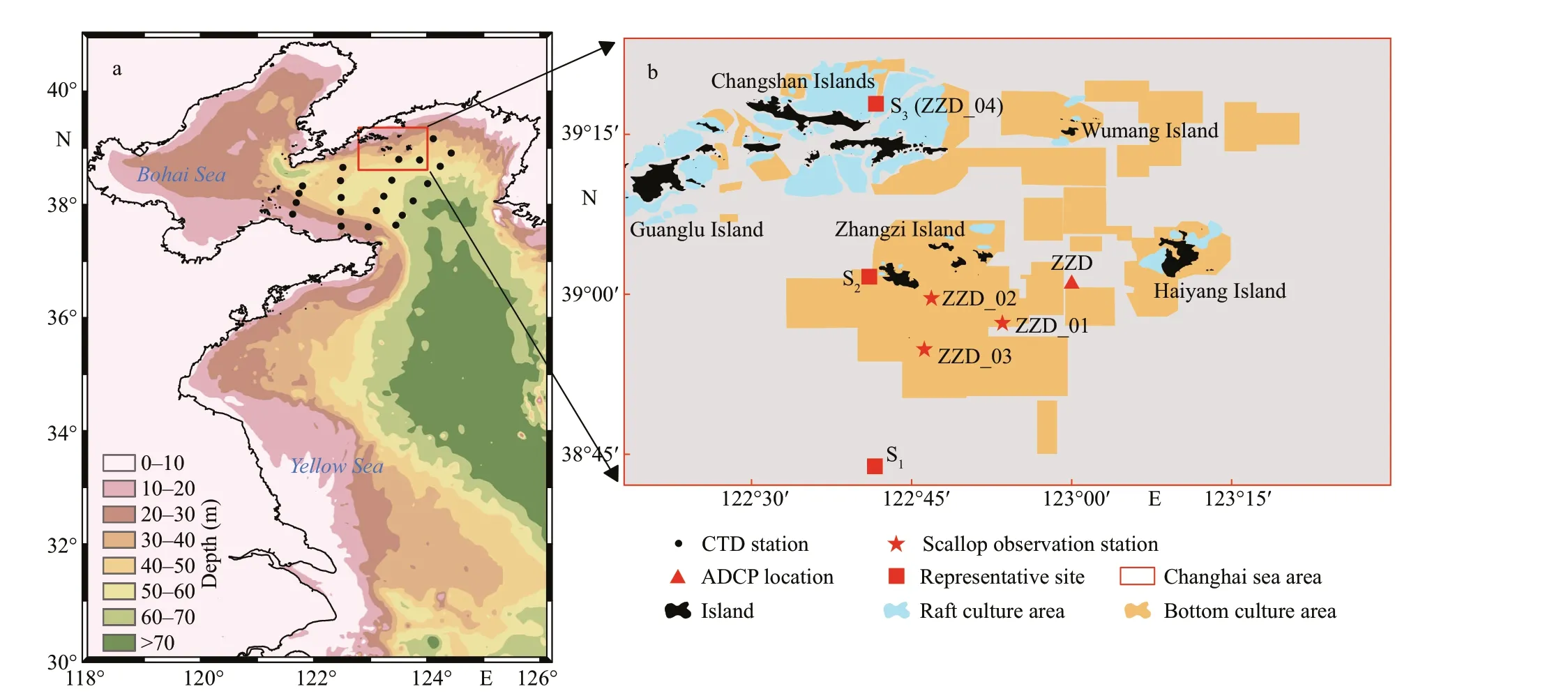
Fig.1 Map of the study area, observation stations, and representative sites

2.2 Overview of the YeSCE model

The Yesso scallop culture ecosystem (YeSCE)model consists of a hydrodynamic model (ROMS), an ecosystem model (CoSiNE), and an offl ine DEB model for Yesso scallop. ROMS and CoSiNE were run simultaneously at 240-s time interval. The realm of ROMS-CoSiNE covered the Bohai Sea (BHS), the Yellow Sea, and part of the East China Sea (Fig.2), in homogeneous 1/24° resolution in horizontal direction and 30 terrain-based vertical levels. Model temperature, salinity, nutrients (nitrate, phosphate,and silicate), and dissolved oxygen were initialized using data from the World Ocean Atlas 2013 V2(WOA13 V2; Boyer et al., 2015). The initial condition for chlorophyllawas prescribed from the hydrodynamical and biogeochemical model NEMOPISCES (Person et al., 2019); and the model was forced with the climatological air-sea f luxes of momentum, wind stress, heat f lux, and freshwater f lux derived from the ERA-Interim reanalysis (Dee et al., 2011). An Orlanski-type radiation condition was applied at the open boundaries for temperature,salinity, and baroclinic velocities (Zhou et al., 2017).The temperature, salinity, water level, and velocity f ields were prescribed using the Hybrid Coordinate Ocean Model (HYCOM; Cummings, 2005)simulation outputs; and the model was forced (data input) at outer boundary by M2, S2, K2, N2, K1, O1, Q1,and P1tide (Luo et al., 2019). Major rivers that surround the study realm in the model included the Changjiang (Yangtze) River, Huanghe (Yellow)River, Liaohe River, Luanhe River, Yalu River,Qiantang River, and Huaihe River in China, and Han River in Korea Peninsula. Monthly-mean runoff of the Changjiang River was used from the measurements at Datong hydrologic station and the monthly-mean nutrient from Global-News model (Wang et al., 2015),while monthly-mean values of the other rivers are taken from previous studies (Zhang, 1996; Liu et al.,2009; Tong et al., 2015). The model consists of 11 state variables, including four on nutrients (phosphate,silicate, nitrate, and ammonium), two on phytoplankton groups (picophytoplankton and diatoms), two on grazers (microzooplankton and mesozooplankton), two on class of detritus (small/suspended and large/sinking), and oxygen. All the state variables are aff ected by physical processes,such as advection and diff usion (Zhou et al., 2017).Phytoplankton, zooplankton, and organic detritus are the main food sources for f ilter scallops (Aya and Kudo, 2010), in the unit of (mmol N)/m3. Using the unit conversion in terms of carbon to nitrogen (C/N)ratio at 6.625 (Redf ield et al., 1963), the food availability in this study was represented as particulate organic carbon ((mg C)/m3). The simulated phytoplankton concentration ((mmol N)/m3) was converted to chlorophyll-aconcentration (mg/m3)using the ratio of 1.58-g chlorophyllaper mole nitrogen (Cloern et al., 1995; Zhou et al., 2017). The chlorophyllawas often used to present the biomass of phytoplankton or the food f iltered and digested by bivalve mollusks (Pouvreau et al., 2006). The rationality of food availability was explained indirectly by verifying chlorophyll-aconcentration.The daily-averaged temperature and food availability of the bottom layer from December 1, 2012 to November 30, 2013 were recorded and used to run the offl ine DEB model.

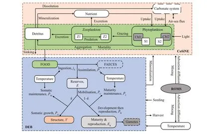
Fig.2 Conceptualization of the YeSCE model

Equations of DEB model were solved using the fourth-order Runge-Kutta numerical integration scheme (Kooijman, 2010) with a time step of 1 day.The DEB model simulates the feeding, digestion,maintenance, maturation, growth, reproduction, and aging processes (Stavrakidis-Zachou et al., 2019), the maintenance energy is def ined as the (mean) energy requirement of an organism, excluding the production processes of growth, reproduction, and development(Kooijman, 2010). These processes are predominantly inf luenced by water temperature and food availability(Kooijman, 2010). The state variables, energy f luxes,and dynamics of the standard DEB model are summarized in Table 1. Two diff erent Arrhenius relationships (K1andK2) were used for scallop ingestion and respiration rates (Bourlès et al., 2009).Most of the key parameters applied in the DEB model were identif ied by previous experiments in Zhangzi Island conducted by Zhang et al. (2016, 2017). Only the half-saturation coeffi cient of food was calibrated.For a more comprehensive description of the DEBtheory and the full list of the equations and the nomenclature, please refer to Kooijman (2010).

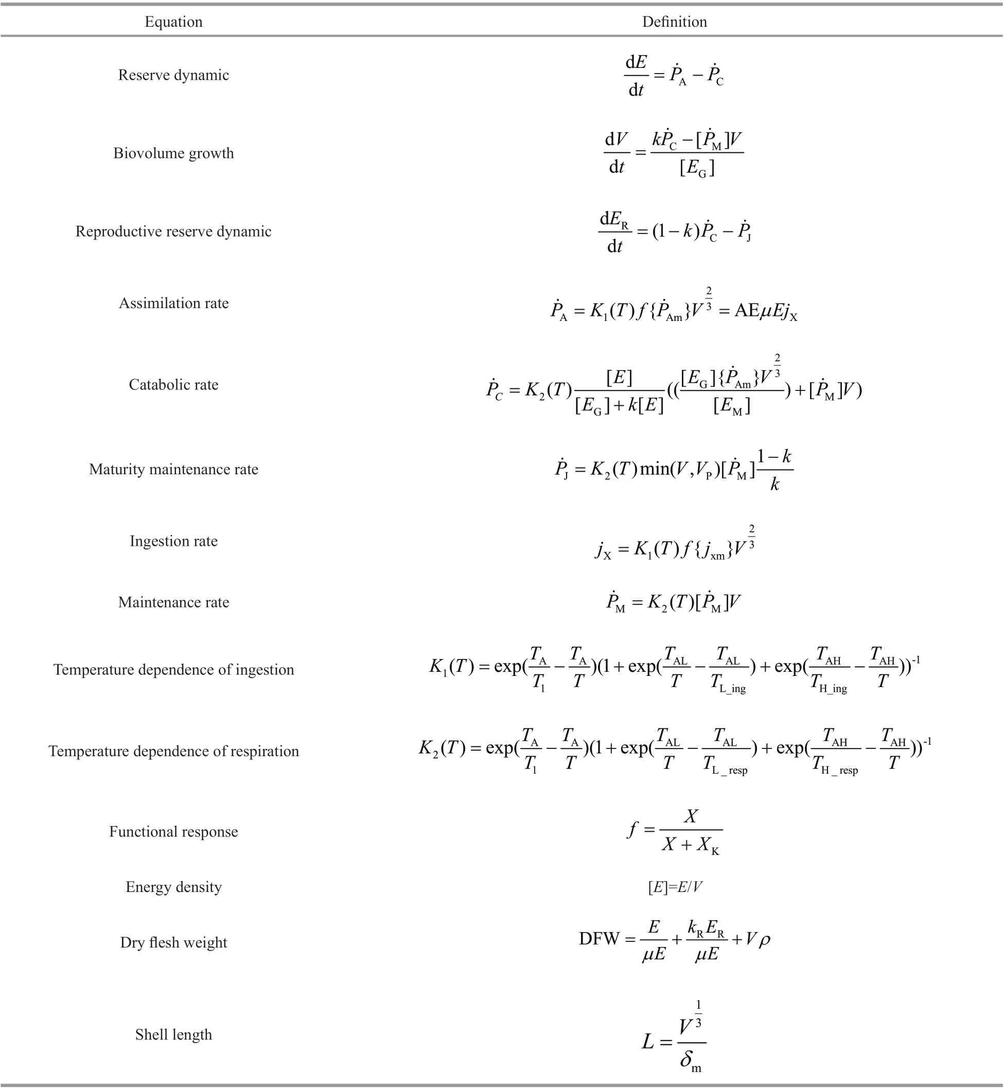
Table 1 Main equations used in the YeSCE model

Fig.3 The observation (blue dots with bars for standard deviation) from December 1, 2012 to November 30, 2014, and the simulation (black line)

2.3 Calibration of YeSCE model

The food uptake of scallops in the DEB model follows Holling’s type II functional response:f=X/(X+XK), whereXis the food availability andXKis the half-saturation coeffi cient, which is the only parameter that requires calibration. Observations of the shell lengths and dry f lesh weights of scallops in station ZZD_01 (Fig.1b; Jiang et al., 2020) were used as the standard. Scallop seeds, with a mean (±SD) shell length of 3.80±0.52 cm and dry f lesh weight of 0.23±0.08 g, were spread abroad the bottom layer on December 1, 2012 (Jiang et al., 2020). The model was calibrated against the f ield observation by minimizing the weighted sum of squared residuals (SSR) using the formulation from Troost et al. (2010). The food availability that corresponds to the minimum SSR was selected as theXKfor YeSCE modeling.

Based on the optimalXK, the observed values of shell length (R=0.97) and dry f lesh weight (R=0.94)exhibited a signif icant correlation with the modeled values. The model can well simulate the growth process of the shell length (Fig.3a) and the change in the energy state of the scallop (Fig.3b).

2.4 Scenario simulation settings

Based on the spatial resolution of the YeSCE model, 810 grid points in the bottom layer in the study area were set up. Yesso scallop seed in each grid point were corresponded with the observations from Jiang et al. (2020), being 3.80 cm in shell length and 0.23 g in dry f lesh weight. The model was run for one year from 1 December 2012 to 30 November 2013 to be consistent with scallop growth data (Jiang, 2013). The model could output the time series of temperature,food availability, shell length, and biomass at each grid point near bottom layer. Biomass is the dry f lesh weight of Yesso scallop in a unit area. The net growth rate refers to the changes in biomass over one year. In the study, we explained the net growth rate as the biomass diff erence from December 1, 2012 to November 30, 2013.

2.5 Suitable growth days

The match-mismatch condition between temperature and food availability aff ects the growth of organisms(Laurel et al., 2011; Scharf et al., 2015). We def ined suitable growth days (SGD) as the number of days of suitable temperature and suffi cient food, which means that the temperature and the food availability were highly matched. The suitable temperature refers to the value in the temperature tolerance range for ingestion(0-20 °C) (Zhang et al., 2016, 2017). Suffi cient food refers to the food availability (X) no less than the halfsaturation coeffi cient (XK).

3 RESULT

3.1 Evaluation of the YeSCE model

3.1.1 Bottom temperature

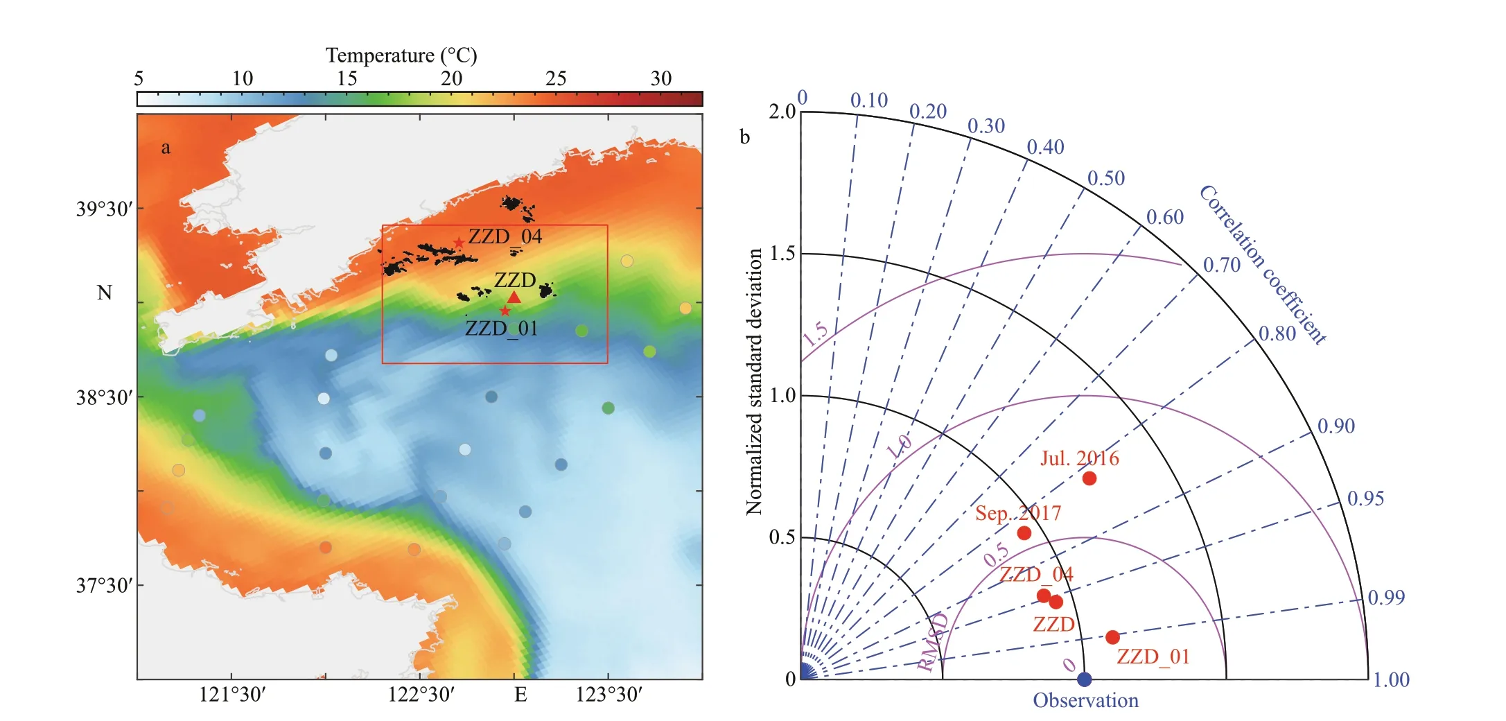
Fig.4 Bottom temperature of simulation (colormap) and observations (dots) on September 10-12, 2017 (a), and Taylordiagram comparing bottom temperature estimates from the observation (blue dot) and the simulations (red dots) (b)

Temperature data shown in Fig.4a were collected with a calibrated CTD (RBR 620) from September 10 to 12, 2017. The distribution of the simulated bottom temperature (background) and observations (points)was consistent, revealing a signif icant correlation between observations and simulations. The model could better reproduce the bottom temperature nearshore than the off shore, and could characterize the cold-water mass and tidal front in the North Yellow Sea (Fig.4a). A more thorough assessment of simulation-observation agreement was conducted quantitatively using the Taylor diagram (Taylor,2001). Temperature data in the bottom layer were from two large-scale surveys in July 9-11, 2016 and September 10-12, 2017, bottom-mooring in station ZZD from July 10 to August 26, 2017, and ZZD_01 from December 2012 to November 2014. The temperature was recorded at 2-m depth in station ZZD_04 from January to December 2007. In addition to the correlation and root mean squared diff erence(RMSD), standard deviations of simulations and observations were calculated in the diagram for each survey (Fig.4b). Note that the standard deviation was normalized by that of observation data to f it all comparisons into one diagram. The correlation between the bottom temperature observation value and the simulation value was signif icant (R＞0.80).Therefore, the model simulated the bottom temperature accurately (Fig.4b).

3.1.2 Bottom chlorophyll-aconcentration

The distribution of chlorophyllafrom YeSCE model matched the CTD (RBR 620) observations from September 10 to 12, 2017. Generally, the simulated chlorophyllain the bottom layer gradually decreased with an increase in the off shore distance(Fig.5a). A more thorough assessment of simulationobservation agreement was conducted quantitatively using the Taylor diagram (Taylor, 2001). Chlorophylladata in the bottom layer were from two large-scale surveys on July 9-11, 2016 and September 10-12,2017, and ZZD_01 from December 2012 to November 2014. Chlorophyllawas recorded at 2-m depth in ZZD_04 from January to December 2007. In the diagram, in addition to the correlation and RMSD,standard deviations of simulations and observations were calculated for each survey (Fig.5b). The statistics showed that the model was capable of modeling chlorophyllain the study area (Fig.5b). The concentration of chlorophyllahas often been used to present the biomass of phytoplankton or food f iltered and digested by bivalve mollusks (Pouvreau et al.,2006). Therefore, an accurate simulation of concentration of chlorophyllais essential to improve the data quality for growth modeling.

3.1.3 Shell length

Based on the observations of Jiang (2013) at stations ZZD_02 and ZZD_03 (Fig.1b), YeSCE model simulated the shell length from December 1,2012 to November 30, 2013. The initial value of shell length was 3.80 cm, which was the same as that in the observation. Reasonable agreement between the simulation results and f ield observation results verif ied the reliability of the model (Fig.6). The modeled shell length results were low in March,mainly due to the insuffi cient food supply from January to March.

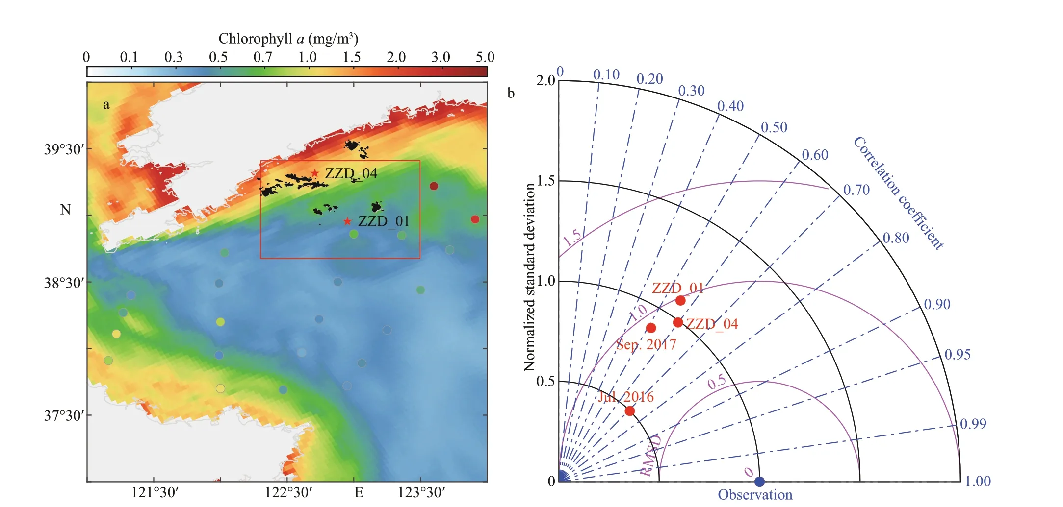
Fig.5 The bottom concentration of chlorophyll a simulated (colormap) and observed (dots) in September 2017 (a), and the Taylor diagram comparing bottom concentration of chlorophyll a estimates from the observation (blue dot) and the simulations (red dots) (b)

3.2 Aquaculture environment

3.2.1 Simulated monthly distribution of bottom temperature

The distribution of simulated monthly average bottom temperature in the study area from December 2012 to November 2013 showed apparent seasonal variations and diff erences from north to south (Fig.7).The simulated temperature in the northern part of the study area changed sharply, with an annual temperature diff erence of more than 28 °C, whereas the diff erence in the southern part of the study area was relatively small. The temperature in the northern shallow-water area was higher than that in the south in summer but lower in winter. The Yellow Sea Cold Water Mass (＜10 °C) aff ected the southern areas with a depth of more than 30 m in June, then gradually retreats to deep-water areas and disappeared in October. The shallow-water area temperature dropped substantially in winter and remained above 4 °C in the deep-water area. In January, the water temperature in the north of the study area dropped to 0 °C. In February and March, it fell into 4 °C. The extreme high/low water temperature in summer/winter could be the major factor that aff ected the scallop growth.

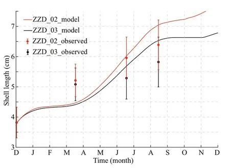
Fig.6 Comparison of simulated (line) and observed (dots with bars for standard deviation) shell lengths in stations ZZD_02 (red) and ZZD_03 (black)

3.2.2 Simulated monthly distribution of food availability

Fig.7 Distribution of monthly averaged bottom temperature from December 2012 to November 2013

The distribution of simulated monthly average food in the study area from December 2012 to November 2013 exhibits seasonal variation (Fig.8).Food availability over the entire study area were lower thanXKfrom November to February, during which shellf ish were restricted by food availability,and grew slowly or stopped growing. The food availability increased from March, peaked in April-May, remained high in June-July, and then gradually decreased. Furthermore, food availability were signif icantly higher in the north than in the south. In the southern deep-water area, the food availability was lower thanXK, which hampered the growth of scallops. High food availability were observed near islands (such as Zhangzi Island). Here, the scallops grow rapidly from April to May (Fig.8e & f) because the food availability was approximately twice that of the surrounding area.

3.3 Simulated distribution of net growth rate

The YeSCE model was applied to the Changhai sea area in the North Yellow Sea to determine the inf luence of natural factors other than the initial seeding density from December 1, 2012 to November 30, 2013. The initial shell length and dry f lesh weight were 3.80 cm and 0.23 g, respectively. The distribution of shell length was high in the north and low in the south, with high values near the islands. At the end of the simulation near Zhangzi Island, the shell length was more than double of the initial shell length up to 8.00 cm (Fig.9a). Similarly, the net growth rate was also the highest near Zhangzi Island (Fig.9b).Therefore, the factors on the spatial diff erence of the net growth rate need to be determined.

The net growth rate refers to the changes in biomass over one year; therefore, the diff erence in net growth rate was inf luenced by biomass in diff erent seasons.Based on the spatial distribution of the net growth rate, three representative sites (S1, S2, and S3, Fig.1b)were selected to analyze the spatial and temporal diff erences of the relationship among temperature,food availability, and scallop growth. Clear diff erence was revealed in biomass contribution from the three representative sites. The biomass of 0.78 g/m2in site S1at the end of the simulation was the lowest among the three sites (Fig.10a). The temperature varied between 3 to 15 °C and food availability was below 60 (mg C)/m3(Fig.10b). At the end of the simulation,the biomass in site S2was 2.60 g/m2(Fig.10d), which was higher than that of S3(2.30 g/m2) (Fig.10g). The duration of temperature lower than 0 °C or higher than 20 °C in site S3was longer than that in site S2(Fig.10e & h). The food availability varied between 25 to 220 (mg C)/m3in site S2, and that of site S3varied between 30 to 300 (mg C)/m3(Fig.10e & h).

Fig.8 Distribution of monthly averaged food availability from December 2012 to November 2013

Fig.9 Distribution of shell length (a) and net growth rate (b)

4 DISCUSSION

4.1 Reasons for the spatial diff erence of net growth rate

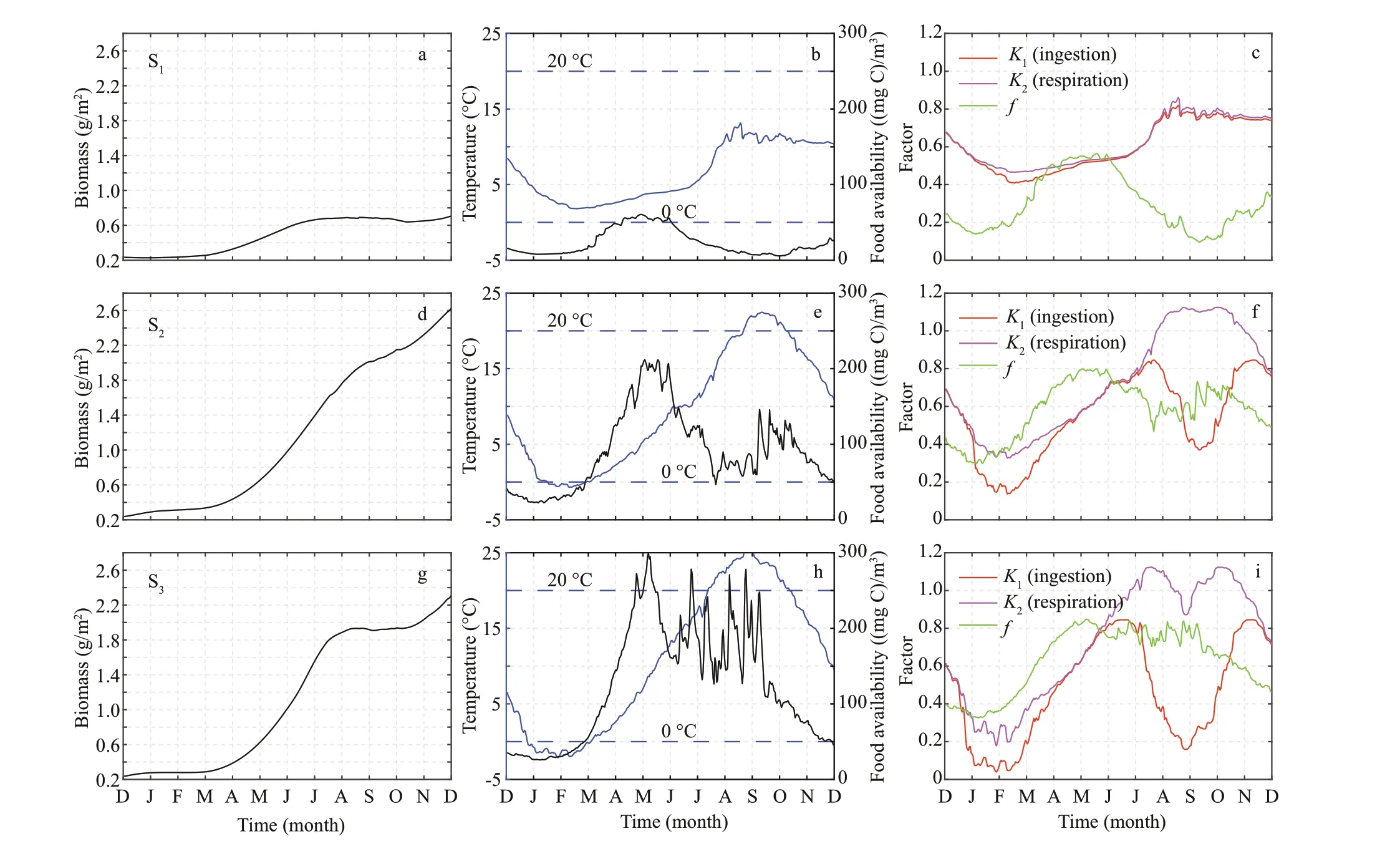
Fig.10 Time series of biomass (a, d, g), temperature and food availability (b, e, h), and factors inf luencing scallop growth (c,f, i) in three representative sites (S 1, S 2, and S 3)

The distribution of net growth rate was high in the north and low in the south, with high values near the islands. The spatial diff erences of net growth rate were the same as the result of the potential for scallop aquaculture development (Liu et al., 2014). It is important to f ind out the reasons for spatial diff erences in the growth rate.fis the dimensionless functional response, which can vary between 0 and 1, and smaller values indicate greater restriction (van der Meer, 2006). The temperature dependence (K1,K2) is a physiological rate at ambient temperature; the smaller the value, the greater the restriction (Bourlès et al., 2009). There was a clear diff erence in the biomass contribution of the three representative sites(Fig.10a, d, & g). Food restriction was the key factor inf luencing the growth of scallops in site S1(Fig.10e).In other words, the low net growth rate area south of the study area was caused chief ly by the lower food availability.

The temperature dependence was the key limiting factor aff ecting the scallop growth in station S2during January to July 2013, which is similar to the previous study near Zhangzi Island (Zhao et al., 2019). The biomass in site S2at the end of the simulation was higher than that of site S3. However, the biomass in site S3(0.40-1.97 g/m2) was higher than that in site S2(0.45-1.84 g/m2) from April to July (Fig.10d & j). In this period, the bottom temperature limitation of the two stations was similar, but the food availability in site S3was almost twice that of site S2(Fig.10e & h).This raises the question of why the biomass was lower in site S3. The reason is that the duration of temperature below 0 °C in site S3was longer than that in site S2from January to March, and the biomass in site S2was 0.45 g/m2, whereas that in site S3was 0.40 g/m2by April. From July to October, the duration of temperature above 20 °C in site S3was longer than that in site S2. In this period, temperature restriction was signif icant. The changes infin the two sites were similar. When the food availability was greater thanXK, the number of days of a suitable temperature determined the f inal biomass of scallops.

4.2 Quantifying the eff ects of food and temperature on scallop growth

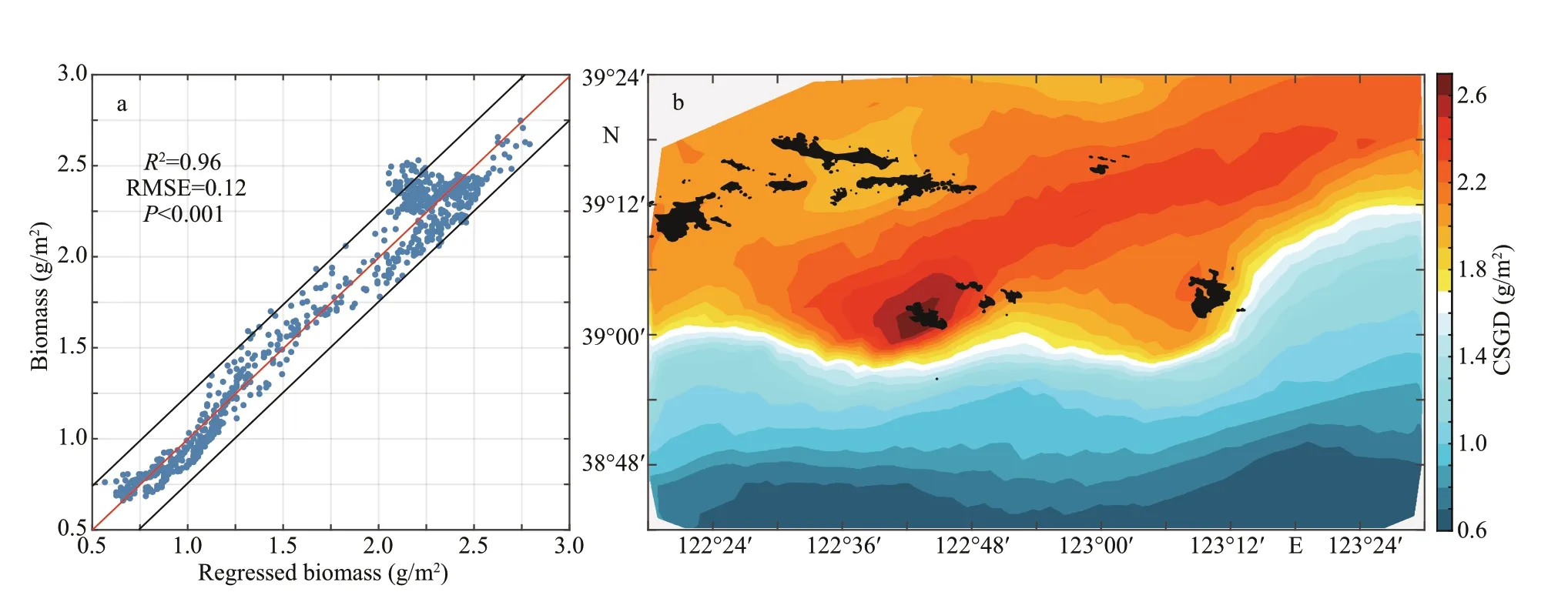
Fig.11 The relationship between regressed and modeled biomass (a) and the contribution of suitable growth days to scallop growth (CSGD) (b)

Based on the relationship between biomass,temperature, and food availability (Fig.10), the match-mismatch condition between temperature and food availability aff ected the growth of organisms(Laurel et al., 2011; Scharf et al., 2015). Meanwhile,the suitable growth days (SGD) represent the number of days during which the temperature and the food availability are highly matched (Laurel et al., 2011).The linear regression of SGD and the biomass at the end of the simulation (BIO) correlates well (BIO=1.19×10-2×SGD+0.14,R2=0.96) (Fig.11a). The equation can be used to express the change in biomass at the end of the simulation. The value 1.19×10-2×SGD represents the contribution of suitable growth days to scallop growth (CSGD). The high-value area of CSGD extends from Zhangzi Island to the northeast of the study area, which is similar to the distribution of the net growth rate. Therefore, the length of SGD is the main factor aff ecting the spatial diff erence in the net growth rate of Yesso scallop.

The contribution of SGD to scallop growth well displayed the spatial diff erences of net growth rate from December 1, 2012 to November 30, 2013(Fig.11), the interannual variation in the scallop growth will be studied in the future. In this study, we considered only the match condition (Laurel et al.,2011) under which the value in temperature tolerance range for ingestion and the food availability (X) is no less than the half-saturation coeffi cient (XK). In other words, we considered that the period of scallop growth were not the slow growth or weight-loss period (Scharf et al., 2015). In the future, we will add mismatch conditions by analyzing the relationship among temperature, food availability, and biomass to make the f itting results more reasonable and f ind out some parameters that are easy to obtain in practice to characterize the spatial diff erences of net growth rate and forecast its interannual variations. Furthermore,YeSCE model can be used to study the interactions between scallop carrying capacity, seeding density,and rotational culture in diff erent regions by changing the initial seeding density and distribution. YeSCE model still needs to be improved in terms of energy dissipation due to biological stress and death due to the invasion of natural predators. Future work should be based on further biological experiments on scallops.

5 CONCLUSION

The YeSCE (Yesso scallop culture ecosystem)model could reasonably simulate the environment and scallop growth in the Changhai sea area. Scallop growth varied seasonally, showing two slow-growth periods from January to March and July to September,which was resulted predominantly from bottom water temperature. The remaining months comprised a fastgrowth period; however, the growth rate from October to December was lower than that from April to June due to food availability. The annual net growth rate was high in the north, low in the south, and notably high near the islands. Based on the correlation analysis, the spatial diff erences of the net growth rate were predominantly aff ected by the duration of suitable growth days.

6 DATA AVAILABILITY STATEMENT

The datasets generated and/or analyzed during the current study are available from the corresponding author on reasonable request.

7 ACKNOWLEDGMENT

The transect observations were collected onboard of R/VDongfanghong2implementing the open research cruise NORC2017-01 supported by the NSFC Ship-time Sharing Project. We acknowledge the crew members of R/VLiaokeyu19from the Zhangzi Island group for their support. We appreciate the help of Simeng QIAN, Chenyi LUO, and Guangyue ZHANG in the preparation of the ecosystem model.