The adjoint-based Two Oceans One Sea State Estimate(TOOSSE)*

Xiaowei WANG , Chuanyu LIU ,4,**, Armin KÖHL , Wu GENG , Fan WANG ,4,Detlef STAMMER

1 CAS Key Laboratory of Ocean Circulation and Waves, Institute of Oceanology, Chinese Academy of Sciences, Qingdao 266071,China

2 Center for Ocean Mega-Science, Chinese Academy of Sciences, Qingdao 266071, China

3 Laboratory for Ocean Dynamics and Climate, Pilot National Laboratory for Marine Science and Technology (Qingdao),Qingdao 266237, China

4 University of Chinese Academy of Sciences, Beijing 100049, China

5 Institut für Meereskunde, Universität Hamburg, Hamburg D20146, Germany

6 State Key Laboratory of Tropical Oceanography, South China Sea Institute of Oceanology, Chinese Academy of Sciences,Guangzhou 510301, China

Abstract An eddy-resolving four-dimensional variational (adjoint) data assimilation and state estimate was constructed for the low- to mid-latitude Pacif ic, Indian Oceans, and South China Sea based on the framework of “Estimating the Circulation and Climate of the Oceans (ECCO)”. It is named as the Two Oceans One Sea State Estimate (TOOSSE). It f its a model to a number of modern observations of 2015-2016,including the Argo f loat temperature and salinity, satellite altimetric sea surface anomalies, by adjusting initial temperature and salinity, sea surface boundary conditions, and background diapycnal diff usivities.In total, ～50% of the original model-data misf its have been eliminated, and the estimated state agreed well with a variety of independent observations at meso- to large scales, and on the intra-seasonal to interannual timescales. Mesoscale variability is systematically strengthened in TOOSSE and closer to observations than that without data assimilation, which is especially evidenced by the improved simulation of the mesoscale tropical instability waves (TIWs). Adjustments to ocean surface forcing parameters exhibit both large and frontal/mesoscale structures, and the magnitude reach 20%-100% of the f irst guesses; the adjustments to diapycnal diff usivity exhibit an obvious elevation (decrement) in (below) the thermocline in the equatorial band. The results indicate that TOOSSE represents a dynamically and thermodynamically consistent ocean state estimate of the 2015-2016 Indo-Pacif ic Ocean, and can be widely utilized for regional process studies.

K eyword: Pacif ic Ocean; Indian Ocean; South China Sea; adjoint; four-dimensional variational data assimilation

1 INTRODUCTION

Via strong modes of variability, e.g., the Indian Ocean Dipole (IOD) and the El Niño-Southern Oscillation (ENSO), the tropical Pacif ic and Indian oceans play an important role in the variability of global climate system. However, in current ocean simulations, either from oceanic general circulation models (OGCMs), or coupled ocean-atmosphere general circulation models (GCMs), remain large model-data misf its at all scales in this region. For example, the area and eastern edge of the western Pacif ic warm pool are far from being correctly simulated (Brown et al., 2014); biases in occurrence,strength and structure of simulated mesoscale eddies exist even using an enhanced grid resolution (Small et al., 2014); the misrepresentation of mesoscale (Ma et al., 2016) and sub-mesoscale (Su et al., 2018) air-sea f luxes could be reasons for the biases. Also, the ENSO prediction skill is limited after 2002 (Clarke, 2014).Those facts indicate strong requirements in better simulating the Pacif ic and Indian oceans. The two oceans are closely connected by exchanging volume,heat and freshwater, as well as by propagated variability information (e.g., Qu et al., 2006; Yuan et al., 2013; Izumo et al., 2014), particularly in the lowto mid-latitude. Therefore, the Pacif ic and Indian Oceans, along with the in-between South China Sea and Indonesian archipelago, should be simultaneously considered as a whole region to derive more accurate state estimates and more comprehensive mechanism analyses.

By optimally combining observational data and ocean models, the adjoint-based four-dimensional variational (4D-Var) data assimilation is recognized as one of the best methodologies to obtain a spatiallytemporally accurate, and dynamically and thermodynamically self-consistent four-dimensional (4D)ocean states. Nevertheless, because of the computational expense, current established ocean state estimates have either global coverage over several decades time but with an eddy-permitting or even lower spatial resolution, e.g., Estimating the Circulation and Climate of the Oceans (ECCO;Stammer et al., 2002), ECCO version 4 (Forget et al.,2015), version 2/3 of the German contribution to ECCO (GECCO2/3; Köhl, 2015, 2020), or with higher resolutions but only on a regional domain and for a short or sometimes segmented assimilation windows. Mazloff et al. (2010) estimated the Southern Ocean state (SOSE) with a 1/6° horizontal grid and 2-year (2005-2006) assimilation window, which provided a description of the freshwater, temperature,and volume transports that are quantitatively consistent with previous inverse estimates. They later produced a 6-year SOSE product at 1/6° resolution(http://sose.ucsd.edu). Verdy and Mazloff (2017)developed a 5-year Biogeochemical Southern Ocean State Estimate (B-SOSE) product at 1/3° resolution that coupled physical-biogeochemical state estimate.Gopalakrishnan et al. (2013a, b) developed a state estimate of the Gulf of Mexico in 2010 with a horizontal resolution of 5-10 km and an assimilation window of 2 months, which was used to initialize the forecast and study the adjoint sensitivity of the loop current evolution and eddy shedding in the Gulf of Mexico. Verdy et al. (2014) produced a long-term window version (4-year assimilation window) of the state estimate of the California Current System State Estimate (CASE) for 2007-2010 on a 1/16° horizontal grid. Zaba et al. (2018) presented a short-time window version (3-months assimilation window) of CASE over the years 2007-2017 and compared it with a network of underwater gliders to assess the estimates with respect to annual and interannual variability in the California Current System. Hoteit et al. (2008)constructed a tropical Pacif ic state estimate and studied the impact of horizontal resolution and optimized ECCO surface forcing on the simulation.Hoteit et al. (2010) carried out an eff ort to bring the model into agreement with a wide variety of observations on 1/3° horizontal resolution for the year 2000. Verdy et al. (2017) built a state estimate over years 2010-2013 with overlapping short assimilation windows (4 months long) for the tropical Pacif ic Ocean at 1/3° horizontal resolution, which obtained good agreement with Tropical Atmosphere Ocean(TAO) mooring observations for time scales shorter than 100 days.

Note, the ECCO Phase II, ECCO2 (Menemenlis et al., 2008), used the Green’s function approach as the assimilation method (Menemenlis et al., 2005). Based on the ECCO2 system, Halpern et al. (2015) assessed the impact of data assimilation on the transports of the Equatorial Undercurrent and the North Equatorial Countercurrent in the Pacif ic Ocean, and Fenty et al.(2017) revealed that synthesizing both ocean and sea ice concentration data is necessary to achieve modeldata consistency of the sea ice in both hemispheres.Carroll et al. (2020) improved the ECCO-Darwin model (Brix et al., 2015; Zhang et al., 2018) which assimilates both physical and biogeochemical observations, and their estimated surface oceanpCO2and air-sea CO2f lux are found consistent with observations in most biomes and over seasonal to multi-decadal timescales.

Yet eff ort is needed to build up a high resolution,and dynamically and thermodynamically consistent ocean state estimate synthesis that simultaneously considers the Pacif ic Ocean, the Indian Ocean, the inbetween South China Sea and Indonesian archipelago as a whole, which consequently can serve as a tool for exploring the inter-basin interactions and multiple scale ocean processes in the Indo-Pacif ic region. This is the objective of the present study. We aim to construct an ECCO-based (with adjoint method)regional synthesis of the low- to mid-latitudes of both the Indian and Pacif ic Oceans. Its horizontal resolution is 1/6°, which is eddy-resolving for the low-latitudes and eddy-permitting for the mid-latitudes. We call this synthesis the “Two Oceans One Sea State Estimate” (TOOSSE). “Two Oceans” stand for the Pacif ic and Indian Oceans while “One Sea” stands for the South China Sea, by which we would like to signify the connectivity, interaction, and integrity of the entire region. As a f irst step, a 2-year long (2015-2016) assimilation window is selected in the present paper. This window length is a compromise between computation cost, suffi ciency of data constraints(which deliver as enough information as possible throughout the model domain), and usability for science. In the future, a longer assimilation window will be tested.

This paper is organized as follows. Section 2 describes the assimilation system, including the model conf iguration, observation constraints, and control variables. In Section 3, the adjusted atmospheric forcing and background vertical diff usivity are analyzed. The estimated state is presented and evaluated in Section 4. Summary and discussion are given in Section 5.

2 METHOD

2.1 State estimate framework

The ECCO framework was adopted to build the TOOSSE synthesis. A brief introduction of this framework is summarized as follow, and more details can be seen in Stammer et al. (2002). Firstly, the consistency between the Massachusetts Institute of Technology general circulation model (MITgcm;Marshall et al., 1997) solutions and the data constrains is measured by a total cost function, which is the sum of all individual cost function contributions. For each individual cost function contribution, the squared diff erences between the model output and the corresponding data constraint (e.g., temperature) or the changes to the control variables (e.g., wind stress;see Section 2.4) are weighted summed over time and space. The weights are the reciprocal of the prescribed error (uncertainty) variance. Secondly, the adjoint model of the MITgcm calculates gradients of the total cost function with respect to a set of control variables.Finally, with those gradients, the quasi-Newton algorithm (Gilbert and Lemaréchal, 1989) determines the adjustments of the control variables according to the descent directions for cost function minimization.The adjoint model of MITgcm was obtained by the algorithmic diff erentiation tool Transformation of Algorithms in Fortran (TAF) (Giering and Kaminski,1998).

We start from a prior ocean state obtained from the forward run of the unconstrained model with the f irstguess of a set of control variables (referred to as the CTRL run hereafter). Then, the control variables are adjusted iteratively to improve the estimation of the ocean state. Finally, when the descent of the total cost function becomes too small to deserve further iterations, the iteration was stopped. The model outputs and the adjusted control variables at the last iteration are considered as the optimized ocean state and the corresponding optimized control variables,respectively.

2.2 Model conf iguration

The domain of TOOSSE ranges from 28°S to 42°N and from 31°E to 69°W (Fig.1). The eastern and western boundaries are closed by the coastlines and the artif icial closure of the Panama and Suez Canals.Open boundary conditions are set at the northern and southern boundaries. The model has a horizontal resolution of 1/6°×1/6°, 50 vertical levels with gradually increasing thicknesses from 10 m near the sea surface to 450 m near the bottom, and a time step of 900 s. Eddies in this low- and mid-latitude region are most prominent with characteristic radius of＜40 km poleward of 30°, of ～40-100 km between 10°and 30°, and ＞100 km equatorward of 10° (Chelton et al., 1998), thus TOOSSE meets the requirement of being eddy permitting in the higher latitudes and eddy resolving in the lower latitudes of this region.

In the forward run, biharmonic horizontal viscosity and diff usivity are used and each was set to 1010m4/s;vertical mixing is represented by the K-Prof ile Parameterization (KPP) scheme (Large et al., 1994),with background vertical viscosity and diff usivity of 10-4and 10-5m2/s, respectively. In addition, background horizontal viscosity and diff usivity coeffi cients are adopted to represent all other unresolved processes,and each was set as 102m2/s. However, to suppress fast exponentially growing modes related to the linearization of nonlinear terms in the forward model,several changes to the adjoint have been made. In the adjoint model, the KPP scheme is excluded, and the background horizontal diff usivity and viscosity values are amplif ied by a factor of 100 similar to the strategy of Köhl and Stammer (2008), Liu et al. (2012), and Verdy et al. (2017).

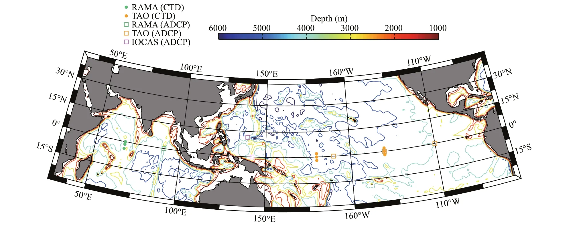
Fig.1 Model domain and bathymetry (in m)

Lateral open boundary conditions are the monthly mean temperature, salinity, and zonal and meridional velocity obtained from the GECCO2 global state estimate (Köhl, 2015). The GECCO2 data covers the period of 1948-2016, and has a horizontal resolution of 1°×1/3° near the equator and 50 depth levels (http://icdc.cen.uni-hamburg.de/1/daten/reanalysis-ocean/gecco2/). A sponge layer is imposed to relax the model thermodynamic variables and to avoid artif icial ref lection. Surface f luxes of momentum, heat and freshwater (salt) are determined with the “bulk formulae” (Large and Pond, 1981, 1982; Large and Yeager, 2004), based on air temperature, air humidity,net precipitation, downward longwave radiation,zonal and meridional wind speed from the 6-hourly NCEP/NCAR reanalysis. The NCEP/NCAR data has a horizontal resolution of about 1.9° and is interpolated onto the TOOSSE grids. Runoff from the 6-hourly ERA-Interim data (Dee et al., 2011; https://www.ecmwf.int/en/forecasts/datasets/reanalysis-datasets/era-interim) is also used.

2.3 Observation data constraints and uncertainty errors

The observational data constraints include sea surface observations from satellite sensors and subsurface observations from Argo prof iling f loats(http://www.argodatamgt.org/). The sea surface height (SSH) data is separated into its mean and anomalies. The mean SSH is the mean dynamic topography (MDT) of the Danish National Space Center DNSC08 (Andersen and Knudsen, 2009)minus its mean averaged over the TOOSSE domain;it has a horizontal resolution of 0.25° and is assigned a homogenous uncertainty of 4.5 cm. The SSH anomalies are adopted from daily sea level anomalies(SLAs) of the along-track altimeter data from Jason-2/Jason-3 (JASON) and CryoSat-2 (ftp://ftp.sltac.cls.fr/Core/SEALEVEL_GLO_PHY_L3_REP_OBSERVATIONS_008_045/). The uncertainties prescribed for the JASON SLAs are half standard deviations of daily JASON SLA data over the period 2010-2016, which are spatially non-uniform and range from ～23 cm in the Kuroshio Extension (KE) to a minimum ～1 cm.To those values, 5 cm is added for the uncertainties of the CryoSat-2 SLAs. The uncertainties are amplif ied by a factor 100 in part of the Indonesian Sea(120°E-130°E, 10°S-10°N), where large corrections always take place and cause computational instability.Considering larger observational errors in coastal areas, SSH observations in locations with water depths less than 500 m are discarded. The monthly sea surface temperature (SST) with a resolution of 1°(obtained from the Hadley Centre Global Sea Ice and Sea Surface Temperature, HadISST; https://www.metoffi ce.gov.uk/hadobs/hadisst/) and monthly sea surface salinity (SSS) with a resolution of 1/5°-1/4°(obtained from the Soil Moisture and Ocean Salinity,SMOS; https://www.catds.fr/Products/Available-productsfrom-CEC-OS/CEC-Locean-L3-Debiased-v3) are used. The uncertainties for SST and SSS are calculated from the Argo data (see below), which range within 0.1-1.5 °C and 0.05-1.10, respectively. The MDT,SST, and SSS data were bi-linearly interpolated onto the TOOSSE grids, while the along-track SLAs were weight-averaged onto the TOOSSE grids using the same method as the Argo prof iles.

For the subsurface layers, monthly temperature and salinity data from quality-controlled Argo prof iling f loats are used. The prof iles were processed onto the TOOSSE grids as follow: a prof ile on the model grid was obtained by weight-averaging all qualif ied Argo prof iles in a 1°×1° box surrounding the grid point, with two-dimension (2D) Gaussian weight coeffi cients that were determined by their distance to the model grid. The obtained prof ile is then averaged onto the vertical model grid. All obtained prof iles occurring in each month are temporally weightaveraged as monthly data, with one-dimension Gaussian weight coeffi cients determined by their distance to the middle date of the month. The prescribed temperature and salinity uncertainties are one standard deviation of the monthly anomalies to climatology of World Ocean Atlas 2013 (WOA13;Locarnini et al., 2013; Zweng et al., 2013; https://www.nodc.noaa.gov/OC5/woa13) within a 1°×1° box surrounding the grid points.

After bringing the original data onto the model grids, the number of observation data constraints used in TOOSSE are about 4.5×105for MDT, 4.3×106for JASON SLA, 6.2×106for CryoSat-2 SLA, 1.1×107for HadISST, 1.1×107for SMOS, 3.9×106for Argo temperature, and 3.9×106for Argo salinity. In addition,the background values for 9 control variables,including the initial conditions, surface forcing, and vertical diff usivity, are part of the constrains via the background terms.

2.4 Control variables

The control variables to be adjusted in the TOOSSE synthesis consist of the 3D initial potential temperature and salinity, time varying air temperature, humidity,zonal and meridional wind speed at 10 m above the sea surface, net precipitation and downward longwave radiation at the air-sea interface, and 3D background vertical diff usivity. The f irst-guess initial conditions are obtained from the GECCO2 at January 1, 2015.The f irst guesses of the sea surface forcing parameters are the 6-hourly NCEP/NCAR reanalysis. The f irstguess background vertical diff usivity isκ0=10-5m2/s.The adjusted diff usivity is formulated asκad=κ0eδκad and hence the adjustment isδκad=κad-κ0=κ0(eδκad-1).The adjustments of the sea surface forcing parameters are made at 3-day intervals. The initial velocities and open boundary conditions were not controlled.

The 9 control variables are also part of the constraints that contribute to the total cost function.The uncertainty of each atmospheric state or f lux f ield was specif ied as the standard deviation of the f ield calculated over 2010-2016, which is the spatially varying f ield. The uncertainty of the diff usivity was prescribed as 10-5m2/s; this choice was based on global estimates of full depth diff usivities (Kunze et al., 2006), which showed values varying by over one order. The prescribed uncertainties of initial temperature (salt) range from 0.52 °C (0.13) near the surface to 0.05 °C (0.01) in deep layers, which were projected from the SSH variability with the Cooper and Haines (1996) scheme. No smoothing operator was used for the control adjustments.

3 ADJUSTMENTS TO CONTROL VARIABLES

3.1 Atmospheric properties

Statistical diff erences between the TOOSSEadjusted atmospheric state f ields and the NCEP/NCAR f ields are shown in Fig.2. Adjustments to zonal wind velocity, downward longwave radiation and precipitation are found at basin scales, while that to the meridional wind are small in the majority of the basins and show some moderate values near the open boundaries and coastal seas. Specif ically, adjustments to the zonal wind velocity (Fig.2a & b) are large in the equatorial bands of the Pacif ic Ocean (with positive sign on average), the southern subtropical Pacif ic(with positive sign on average), the eastern boundary of the Indian Ocean along the Indonesian Islands(with negative sign on average), the Kuroshio Current(KC) and KE (with negative sign on average), and the Luzon Strait (with positive sign on average). In some of these regions the adjustments exceed 5 m/s,comparable to the magnitude of the f irst guess. The mean adjustments are within the range of 1 to 4 m/s,～10%-100% in magnitude of the f irst guess and comparable to the prescribed uncertainties. Large mesoscale adjustments are found in eddy-rich regions where strong instabilities exists, such as the northern front of the cold tongue in the eastern Pacif ic, the southern edge of the South Equatorial Current (SEC)in the central Pacif ic, and the KC and KE (Fig.2a &b). Adjustments to meridional wind velocity are nearly zero in most regions, but show f luctuating pattern along the northern open boundary and coastal regions (Fig.2c & d).

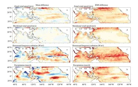
Fig.2 Statistical diff erences of atmospheric state f ields between the TOOSSE and the NCEP/NCAR

Fig.3 The 3-day adjustments to atmospheric forcing f ields during Sep. 5-7, 2016

Both large scale and mesoscale adjustments are obtained for the downward longwave radiation(Fig.2e & f). The adjustments are negative in the central and eastern equatorial Pacif ic, and the western equatorial Indian Ocean; yet positive over most of the tropical and subtropical region, including the maritime continent. The mesoscale adjustments occur mainly off the equator of the Pacif ic and along the eastward portion of the subtropical gyre in the southern Pacif ic.The adjustments reach over 100 W/m2(also refer Fig.3c), comparable to the magnitude of f irst guess which is ～100-400 W/m2.

Adjustments to the precipitation (Fig.2g & h) show a large-scale pattern. They are generally positive in the northwestern and southeastern Pacif ic, as well as in the western and southern tropical Indian Ocean.Negative adjustments are in and surrounding the maritime continent, within 0°-10°N of the central and eastern Pacif ic, in the Bay of Bengal, and near the eastern coastal of Australia (also refer Fig.3d). Both positive and negative adjustments have a maximum exceeding 4 mm/day.

Although the overall mean adjustments to the atmospheric variables are moderate, the local mesoscale adjustments are strong and show prominent spatial variations (Fig.3). The mesoscale adjustments are obvious compared to the atmospheric state adjustments determined by the lower-resolution GECCO2, which, however, shows similar large-scale patterns. These mesoscale adjustments may signif icantly impact the simulated ocean state and effi ciently bring it into consistency with observation data constraints. A similar f inding was also reported by Mazloff et al. (2010) for SOSE.

3.2 Background vertical diff usivity

We f irst choose a central depth of a model layer(174 m) which covers the upper thermocline layer of most of the study region, to show the adjustments to the background vertical diff usivityδκad. Figure 4a shows that large positive adjustments (with the same order of magnitude as the background value) occur in the equatorial bands of the two oceans and in the Arabian Sea. Moderate positive adjustments happen in the Bay of Bengal, the South China Sea, and the eastern Northern Pacif ic, while weak negative adjustments occur in the tropical South Pacif ic.

δκadwas further illustrated in two vertical sections,one along the Equator and the other along 160°E in the western Pacif ic. The equator section (Fig.4b) also exhibits signif icant positive adjustments in the thermocline of the Pacif ic Ocean, the Indian Ocean,and the Indonesian seas. Here, the elevated mixing may represent the eff ect of the small vertical scale(O(10) m) shear instability caused by inertial instability oscillations (Richards et al., 2012), and the combination of large scale currents with low mode equatorial waves (Zhu et al., 1998) or inertio-gravity/near-inertial oscillations (Alford and Gregg, 2001;D’Orgeville and Hua, 2005). Particularly, the enhanced vertical mixing in the equatorial thermocline of the eastern Pacif ic has been observed (Peters et al.,1991; Gregg et al., 1996; Moum et al., 2009) and argued to be associated with the combined strong shear from both the Equatorial Undercurrent (EUC)and the tropical instability waves (TIWs) (Moum et al., 2009; Liu et al., 2016, 2019a, b).

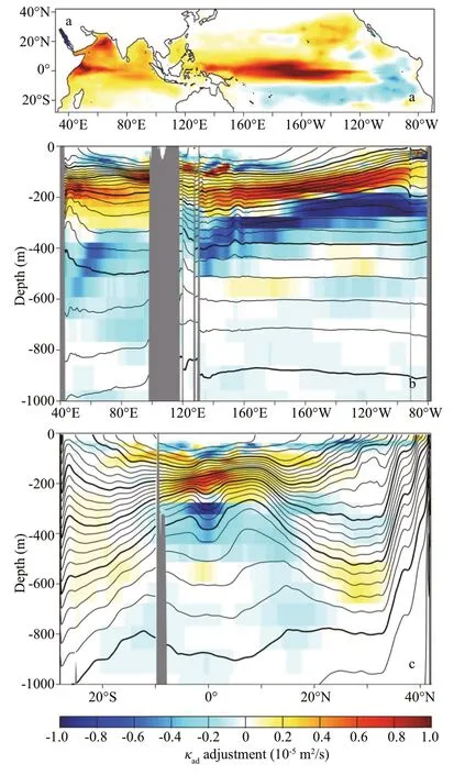
Fig.4 Adjustment to the background vertical diff usivity

The meridional section (Fig.4c) shows a representative north-south equatorial symmetry between 20°S and 20°N, with cores of large positive adjustments at depths of 100-250 m. It also shows another apparent core of positive adjustment near 28°N-29°N of the main thermocline (500-700 m),which verif ies the widely reported elevated mixing induced by the parametric subharmonic instability(PSI) mechanism taking place between the semidiurnal internal tides and inertial frequency(Mackinnon and Winters, 2005; Alford et al., 2007;Simmons, 2008; Qiu et al., 2012; Mackinnon et al.,2013). It’s also clear that large negative adjustments occur in the mixed layers (above 100 m) and at the lower part of the thermocline (～250-450 m). This feature indicates that the background vertical diff usivity is overestimated in these layers. The weakened diff usivity in lower thermocline layers could be of dynamical importance. For example,Furue et al. (2007, 2009) argued that the Equatorial Intermediate Current (EIC) could be reproduced only with very weak or no interior diff usion in OGCMs.The adjustments thus have potential impacts on how the EIC is reproduced. Below 800 m, however, there are nearly no adjustments. We note that no adjustments may not suggest that the f irst guess is proper; instead,it may indicate that those regions are not suffi ciently sensitive to vertical diff usivity changes on the 2-year timescale of the integration.

4 ESTIMATED STATE

4.1 Optimization

The optimization can be examined by the iterative evolution of the normalized individual cost function contribution, which is calculated as the root of the cost function divided by the total number of data points of this data type. Take Argo temperature (T) for example, its normalized cost functionCTis calculated as

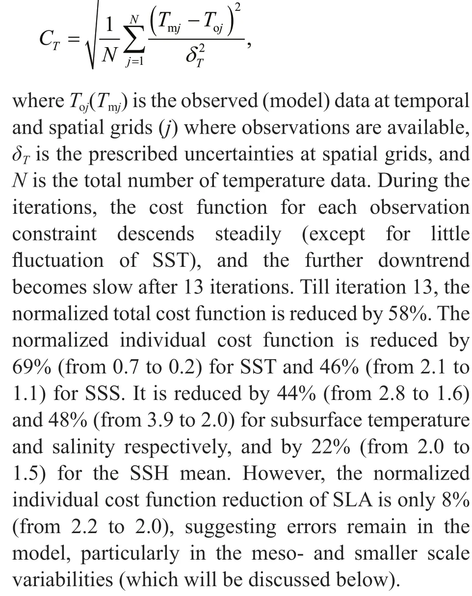
Values of most normalized individual cost function range between 1 and 2 (except for that of SST which is 0.2), indicating that the mean bias between model state and data constraints is 1-2 times of the prescribed uncertainties. These values are within the range of previous products (e.g., Köhl, 2015; Verdy et al.,2017) and considered acceptable. Indeed, the large descent of total cost function has evidenced that the estimated state is signif icantly improved in TOOSSE.In the following, we will show that the solution of TOOSSE has also been brought into good agreement with independent data. The comparison between CTRL (without data assimilation) and TOOSSE (the optimized state based on iteration 13) is also presented below.

4.2 Comparison with data constraints

4.2.1 Mean temperature and salinity

The mean biases and root mean square (RMS)diff erences of SST between model solutions (CTRL and TOOSSE) and the HadISST are shown in Fig.5.Large SST errors of CTRL mainly exist along the main oceanic fronts, such as the eastern part of the Equatorial currents, the Peru Current, the KC and KE,as well as the Indonesian throughf low (ITF), with a maximum exceeding 2 °C (Fig.5a & c). In comparison to CTRL, the error from TOOSSE is greatly reduced over the whole domain; in the above mentioned areas where the errors are relatively large in CTRL, the improvement can exceed 1.5 °C. The estimated SST shows quite small mean biases of less than ±0.2 °C and RMS diff erences of less than 0.4 °C in about 70%of the domain. However, there are still large biases and RMS diff erences exceeding 1 °C in some areas,such as north of 30°N of the Pacif ic Ocean. In these regions, the TOOSSE is only able to marginally resolve the eddies. A great improvement is also obtained for the SSS (Fig.5e-h), with quite small remaining mean biases of less than ±0.1 and RMS diff erences of less than 0.2 in about 80% of the domain. The results demonstrate that TOOSSE has achieved a signif icant improvement in simulating the SST and SSS.

The temperature and salinity in subsurface layers downward to 2 000-m depth also gain considerable improvements by TOOSSE. The domain and time mean prof iles of biases and RMS diff erences with respect to the Argo data for CTRL and TOOSSE are shown in Fig.6. Prof iles of temperature bias and RMS diff erences of TOOSSE have almost the same vertical structure as that of CTRL, except for the opposite bias above 90 m. However, compared to CTRL, the bias of TOOSSE is reduced throughout the whole water column, with an average decrease of 0.15 °C and a largest reduction of over 0.4 °C between 100 m and 250 m. Also, RMS diff erences between TOOSSE and Argo drop by values ＞0.5 °C in the upper 400 m to values ＜0.17 °C below 1 000 m. Overall, after optimization, the temperature bias becomes quite small below 450 m, though remains between -0.16 °C and 0.23 °C above.

The improvement in salinity is shown in Fig.6b.Compared with CTRL, the bias of TOOSSE salinity is reduced throughout almost the whole water column, and notably the bias approaches nearly zero below 400-m depth. The RMS diff erences of TOOSSE are also reduced over the whole water column, with gradually decreasing reductions from a maximum of 0.12 at surface to less than 0.02 below 1 000 m.

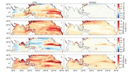
Fig.5 Comparisons of SST and SSS between the model solutions and the assimilated data

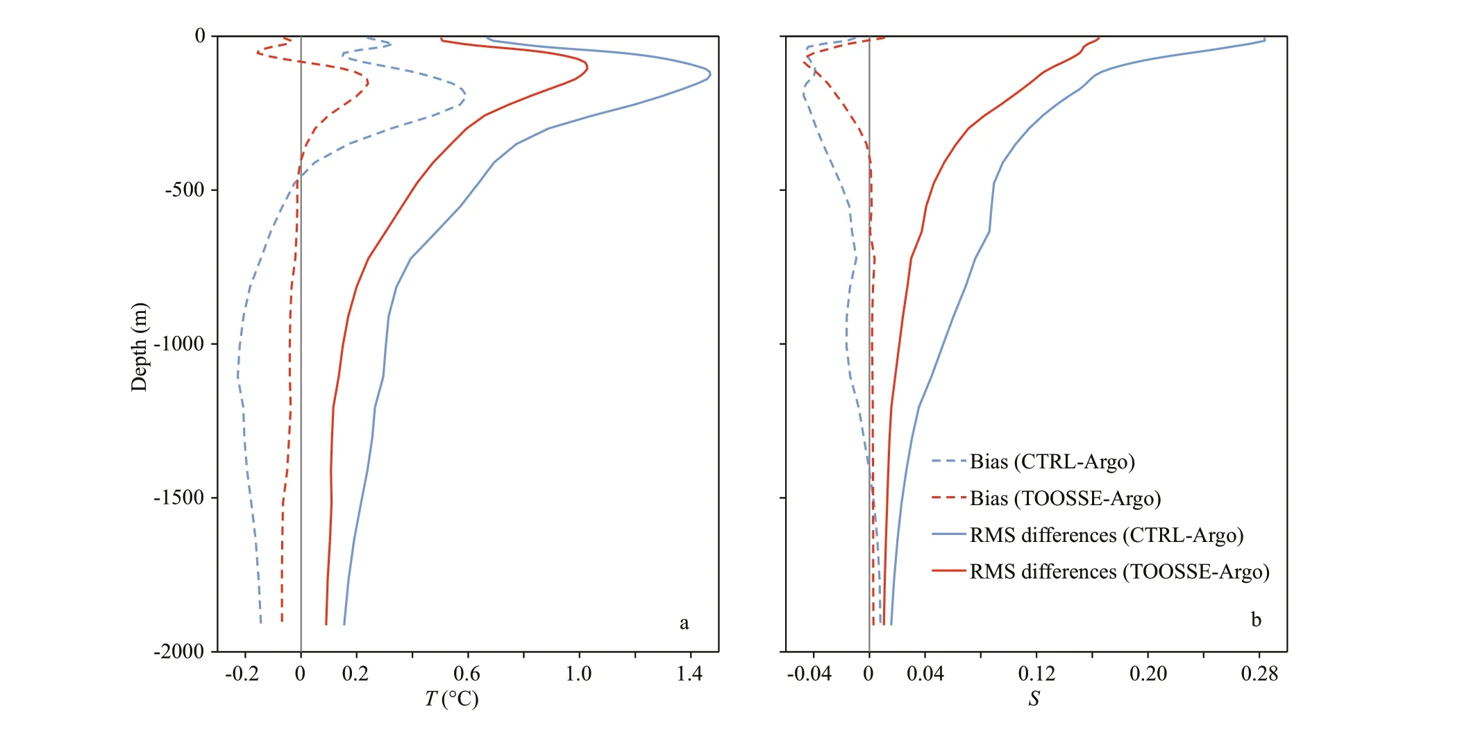
Fig.6 Comparisons of the domain and 2-year mean temperature (in °C) (a) and salinity (b) between the model solutions and the Argo data

4.2.2 Mean SSH and SLAs

Fig.7 Daily mean SLA (in m) on Oct. 15, 2016 and mean SSH (in m) from the AVISO data, the CTRL, and the TOOSSE

The SSH ref lects the integrated eff ect of the temperature and salinity throughout the whole water column, and therefore has an important role in validating the estimate. Here, we compare TOOSSE to the gridded AVISO products (http://www.marine.copernicus.eu), including the SLAs and mean SSH.The AVISO data is on a 0.25°×0.25° grid, and its daily SLA and 2-year mean absolute dynamical topography(ADT) over 2015-2016 is taken for comparison. We note that TOOSSE is not directly constrained to these AVISO products, but to the along-track altimeter observations and the MDT of DNSC08. However,since the gridded AVISO SLA and ADT datasets are also made from the along-track altimeter observations,they serve as dependent data here. The mean SSH distribution of the TOOSSE (Fig.7f) is more consistent with that of the AVISO (Fig.7d) than that of the CTRL(Fig.7e). Compared with the AVISO SLAs (Fig.7a-c),TOOSSE also shows better performances than CTRL(note that the 2015-2016 means of the SSH were f irst removed from each data set). TOOSSE not only captures the large-scale pattern of AVISO, such as the opposite sign of SLAs on and off the equatorial region, the high levels of eddy activity in the subtropical North Pacif ic and on the east and west sides of the Australia, but also captures the strong mesoscale variabilities in the eastern tropical Pacif ic,where eddies and the TIWs exist. However, diff erences in the numbers, sizes, intensities, and locations of eddies still remain.

To compare the time variability of the model SLAs against AVISO, we show daily SLA time series at nine sites, located on the equator and 15°N/S of the eastern Indian Ocean and the western and eastern Pacif ic Ocean, in Fig.8. The f igure demonstrates that TOOSSE can capture the multiple temporal scale variations from the year-to-year diff erence over seasonal variability to intra-seasonal variations. It also demonstrates that TOOSSE produces more accurate intra-seasonal variabilities than CTRL in most of the locations. However, there are still some deviations in the intra-seasonal oscillations of TOOSSE, such as the smaller amplitude in the northern Pacif ic Ocean and the larger amplitude in the southern Indian Ocean, which are probably due to the energy damping with the lack of resolution in the forward model. Generally, we see that the SLAs simulated by the TOOSSE show good agreement with the AVISO data.

4.3 Evaluation with independent data

Now we evaluate TOOSSE with independent data that were not assimilated into the synthesis. We choose the temperature and the currents in terms of the two-year mean state, year-to-year (EI Niño to La Niña) and intra-seasonal (mesoscale) variations for the evaluation. In the “Two Ocean One Sea” region,two important observation systems exist: the Tropical Atmosphere Ocean/Triangle Trans-Ocean Buoy Network (TAO/TRITON) mooring array in the Pacif ic Ocean, and the Research Moored Array for African-Asian-Australian Monsoon Analysis and Prediction (RAMA) in the Indian Ocean (http://www.pmel.noaa.gov/gtmba/). These mooring arrays have been observing a number of atmosphere and ocean variables from sea surface to 750-m depth since 1979 for TAO/TRITON and since 2000 for RAMA, supporting monitoring and prediction of multi-scale variations in the tropical Pacif ic and Indian Oceans.

4.3.1 Time varying temperature at diff erent levels

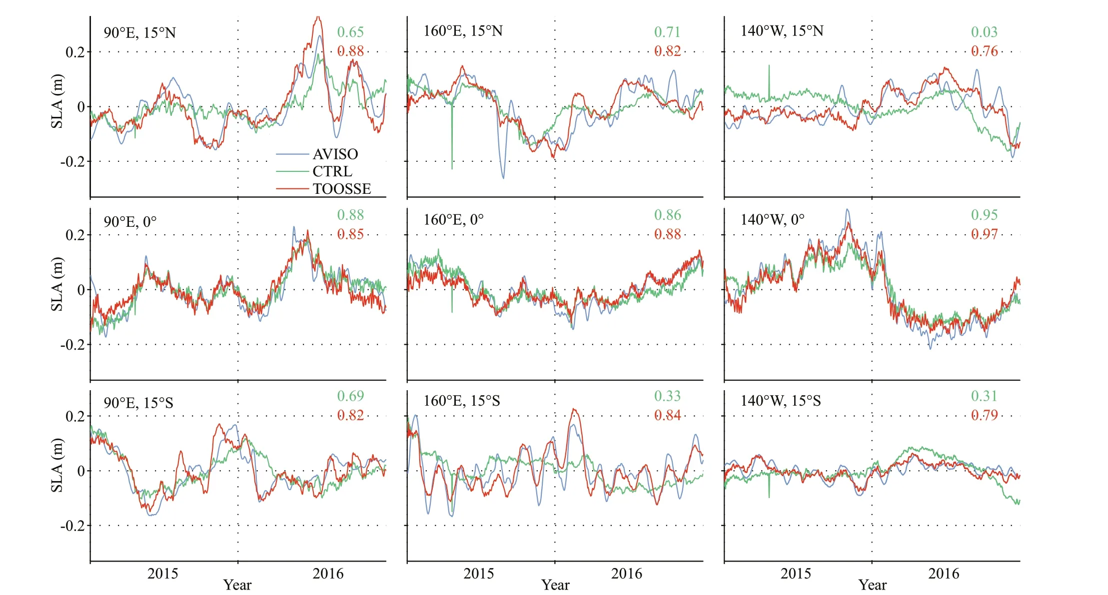
Fig.8 Time series of daily SLAs (m) from the AVISO data (blue), the CTRL (green) and the TOOSSE (red) at sites located in the eastern Indian Ocean (left column), central Pacif ic (middle column), and eastern Pacif ic Ocean (right column),respectively

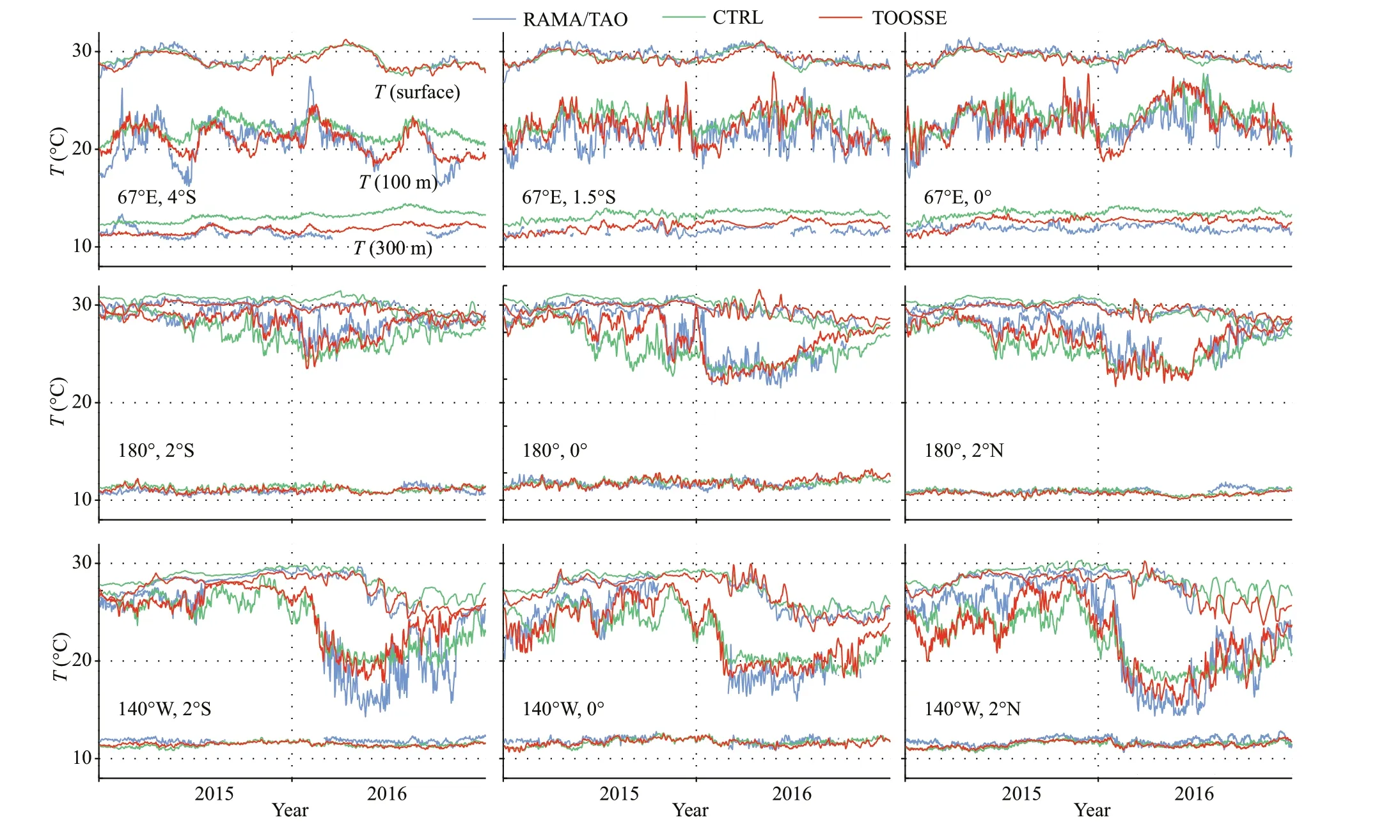
Fig.9 Time series of daily temperature (in °C) from the RAMA/TAO data (blue), the CTRL (green), and the TOOSSE (red)

The daily temperature at the surface, 100-m and 300-m depths from nine sites (Fig.1) of those two observation systems are chosen (Fig.9). In the equatorial Indian Ocean (67°E), the central (180°E)and eastern (140°W) Pacif ic Ocean, temperature at the three levels from TOOSSE match the observations well on both the annual and seasonal scales; the bias between TOOSSE and the observations is modest(with mean RMS diff erences of 0.9 °C) over the two years for all sites. Particularly, the TOOSSE temperature at the surface layer shows a good agreement with the observations. Generally, the overall variability at intra-seasonal and longer scales is well simulated, and the signif icant diff erences between the EI Niño year (2015) and the La Niña year(2016) are accurately captured in both oceans. In most time periods and at all nine sites, TOOSSE’s results are generally closer to observations than CTRL.However, misf its remain: in the central thermocline(～100 m) where the temperature f luctuations are rapid, the intra-seasonal discrepancies are large in some time periods (e.g., the f irst half of 2015); the water is generally colder in the El Niño year (2015)and warmer in the La Niña year (2016) in the eastern Pacif ic. The discrepancies in the western and eastern tropical Pacif ic are larger than those in the central Pacif ic, owing to the relatively more complex multiscale processes in the former regions, such as the meandering boundary currents, TIWs and mesoscale eddies.

4.3.2 Mean subsurface currents and variabilities

Figure 10 shows the simulated time-mean(averaged over the same time period as the observations) and standard deviation (STD) prof iles of subsurface zonal currents against moored Acoustic Doppler Current Prof iler (ADCP) observations at six sites (Fig.1). These observation data are obtained from the TAO/TRITON, the RAMA, and by the Institute of Oceanology, Chinese Academy of Sciences (IOCAS). Additionally, the mean zonal velocities of TOOSSE are also shown on the meridional sections where these mooring sites are located. In the upper layers of the tropical Pacif ic, the main f lows include: a) the eastward EUC, which is centered on the equatorial subsurface layers, relatively shallower in the eastern Pacif ic and deeper in the western Pacif ic (Fig.10c-f); b) the eastward North Equatorial Countercurrent (NECC) at 5°N-10°N and 0-100 m (Fig.10d-f); c) the westward SouthEquatorial Current (SEC) at 10°S-4°N and 0-100 m(Fig.10d-f); d) the westward North Equatorial Current(NEC), which is centered around 13°N (Fig.10b). It's shown that all the main currents are well simulated by the TOOSSE synthesis. TOOSSE also reproduces the main currents in the tropical Indian Ocean: the eastward Equatorial Countercurrent (8°S-2°N) and the westward South Equatorial Current (18°S-8°S) at 0-100 m (Fig.10a, right panel). These results demonstrate that the TOOSSE synthesis has the skill to reproduce the main current system of the domain.However, there also exist systematic quantitative discrepancies in the simulated mean zonal f lows. In the Pacif ic (Fig.10c-f), diff erences in both the mean and the STD of the EUC between TOOSSE and observations exceed 20 cm/s at some depths. The westward EIC observed by Johnson et al. (2002),which was below the EUC in the western part of the Pacif ic, does not appear in TOOSSE (Fig.10c). The EIC is found to be diffi cult to reproduce by OGCMs without carefully tuned (generally reduced)background vertical and horizontal diff usivities(Furue et al., 2007, 2009; Verdy et al., 2017).

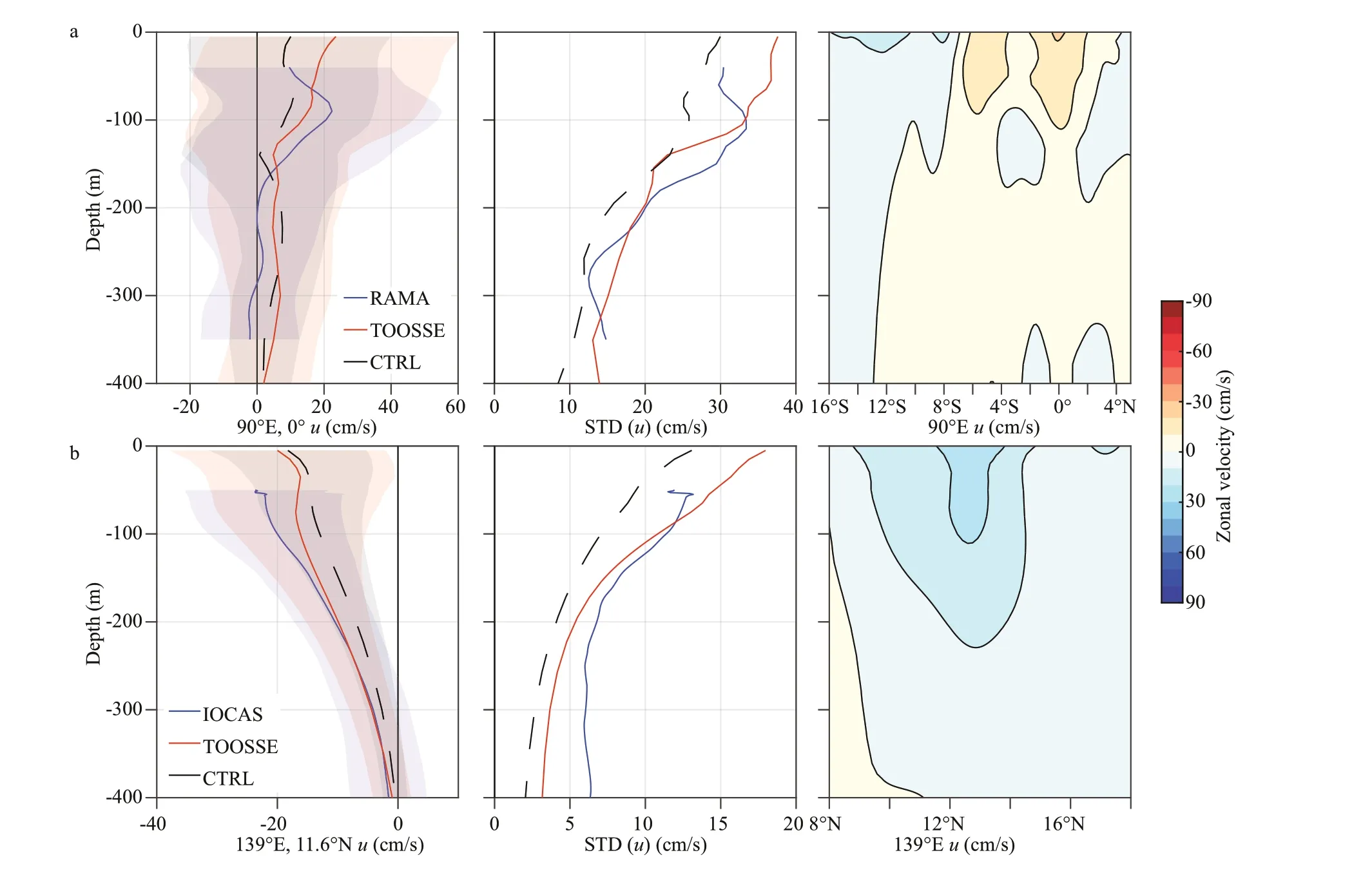
Fig.10 Time mean prof iles (left panel of each set), the corresponding standard deviation (STD) prof iles (middle panel of each set), and meridional sections (right panel of each set) of zonal velocities (in cm/s) from the mooring ADCP observations (blue), the CTRL (black), and the TOOSSE (red) at diff erent sites

To be continued

Fig.10 C ontinued

Specially, TOOSSE-estimated zonal velocities at site 140°W, 0°N, which match the TAO observations quite well, are also compared with those from three reanalysis data: the HYCOM (1/12° resolution;Bleck, 2002; https://www.hycom.org/dataserver/gofs-3pt0/analysis), ECCOv4r4 (1/2° resolution;Forget et al., 2015; https://ecco.jpl.nasa.gov/products/v4r4/) and GECCO2 (Fig.10e). It clearly demonstrates that there are large discrepancies exist in both CTRL and three reanalysis data, while TOOSSE better f its the mean vertical structure and the time variabilities of the zonal velocity at this site than those simulations.

In comparison with CTRL, it is noticed that TOOSSE seems to have little advantages in terms of the mean velocity. For example, their mean zonal velocities at 170°W, 0°N are almost identical (Fig.10d& e), and CTRL is even better at a few depths of other sites. Nevertheless, TOOSSE has a systematically stronger velocity variability than CTRL, which is closer to observations at all sites except for 142°E,0°N (Fig.10, middle panels of each set). This suggests that TOOSSE improves the mesoscale and intraseasonal simulations of currents.

4.3.3 Mean surface currents

Now we present the 2-year mean sea surface (the f irst layer of TOOSSE) currents (Fig.11). The employed independent data are the surface horizontal currents averaged over 2015-2016 from the Ocean Surface Current Analyses Real-time (OSCAR)database (Lagerloef et al., 1999; https://podaac.jpl.nasa.gov/dataset/OSCAR_L4_OC_third-deg). The OSCAR currents have a resolution of 1/3° and are calculated from the satellite-sensed sea surface height gradients, winds and sea surface temperature and are based on the geostrophic relation, the Ekman transport theory, and the thermal wind balance. It shows that the TOOSSE mean surface currents are generally consistent with OSCAR. The basic currents in the Pacif ic Ocean (such as the NECC, SEC, NEC, the KC and KE), the Indian Ocean (such as the eastward Equatorial Countercurrent, the westward South Equatorial Current, and the Somali Current), and the South China Sea, are all well reproduced. In contrast,CTRL produces too weak equatorial currents and too smooth f low f ields of the KE.

Discrepancies of TOOSSE exist mainly in the ITF and western boundary currents of the tropical Pacif ic,which are weaker in TOOSSE compared with those of OSCAR. In addition, the subtropical circulation in the southeast Pacif ic of TOOSSE is a bit stronger than that of OSCAR. The discrepancies in the ITF are likely due to the insuffi cient spatial resolution for the narrow channels and the complex topography of the Indonesia Archipelago, or possibly inaccurate prescription of the throughf low via open boundary conditions, and/or from the calculation errors of OSCAR in regions near the equator. The misf its northeast of the Papua New Guinea, west of the Peru,and along the KC in the East China Sea are probably owing to inaccurate wind forcing in those coastal regions, where fewer data constrains were available for correction and insuffi ciently resolved topography may also cause additional misf it. Further eff orts need to be made to improve the surface currents simulation in the above regions.

4.4 Improved simulation of the TIWs

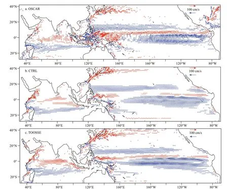
Fig.11 Two-year mean surface horizontal current from the OSCAR data (a), CTRL (b), and TOOSSE (c)

In this section, we choose the TIWs in the eastern tropical Pacif ic as an example for exploring the improved simulation of a specif ic ocean process in TOOSSE. Choosing TIWs has several advantages.Firstly, the latitude of the TIWs’ center is relatively steady (4°N-5°N at the northern edge of the Pacif ic cold tongue) compared to the random mesoscale eddies in the oceans; secondly, their size is relatively large (with a wave length of ～10°) and can be well captured by both observations and OGCMs; thirdly,their strength is related to the background currents as well as the air-sea f luxes (Zhang and McPhaden,1995; Liu et al., 2000; Thum et al., 2002; Pezzi et al., 2006; Seo et al., 2007; Zhang and Busalacchi,2008; Small et al., 2009; Wei et al., 2018, 2019;Zhang, 2014, 2016). However, we note that by TIW we refer to the normally recognized one which is centered at ～4°N-5°N. This wave is strong enough so that it forms a vortex between the Equator and～10°N, which is also referred to as tropical instability vortex (TIV, Flament et al., 1996; in the meanwhile,a diff erent TIW can occur at the Equator which is referred as the equatorial mode TIW or eTIW, Liu et al., 2019b). TIWs are found to have signif icant interannual variability, which is strong and prominent in La Niña years, and weak or even absent in EI Niño years (e.g., Liu et al., 2016). In our simulations,we do have weak TIWs in 2015 (EI Niño year) and strong TIWs in 2016 (La Niña year). For instance,on Sep. 6 of 2016, the observed three mature anticyclone vortexes (Fig.12a & b) with larger SSH than the surrounding water in the chosen area 160°W-120°W were also prominent in TOOSSE(Fig.12e & f).

Compared to CTRL, simulation improvements by TOOSSE are obvious for all the properties of the TIWs. First, the time evolution of SLAs (Fig.13) and the magnitudes of either zonal or meridional velocity anomalies at the equator (Fig.14e & f) associated with TIWs in TOOSSE are closer to the observations(Figs.13, 14a & b). In contrast, the variability of CTRL (Figs.13, 14c & d) is systematically smaller than that of TOOSSE or the observations, while the TIWs produced by HYCOM are rather too strong(Fig.14g & h). Secondly, TOOSSE’s TIWs in year2016 better developed and matched the observed TIWs almost in phase (Figs.12 & 13). In addition,TOOSSE also produced the best background mean current of the SEC and EUC above the equatorial thermocline in the TIWs region (Fig.10e).

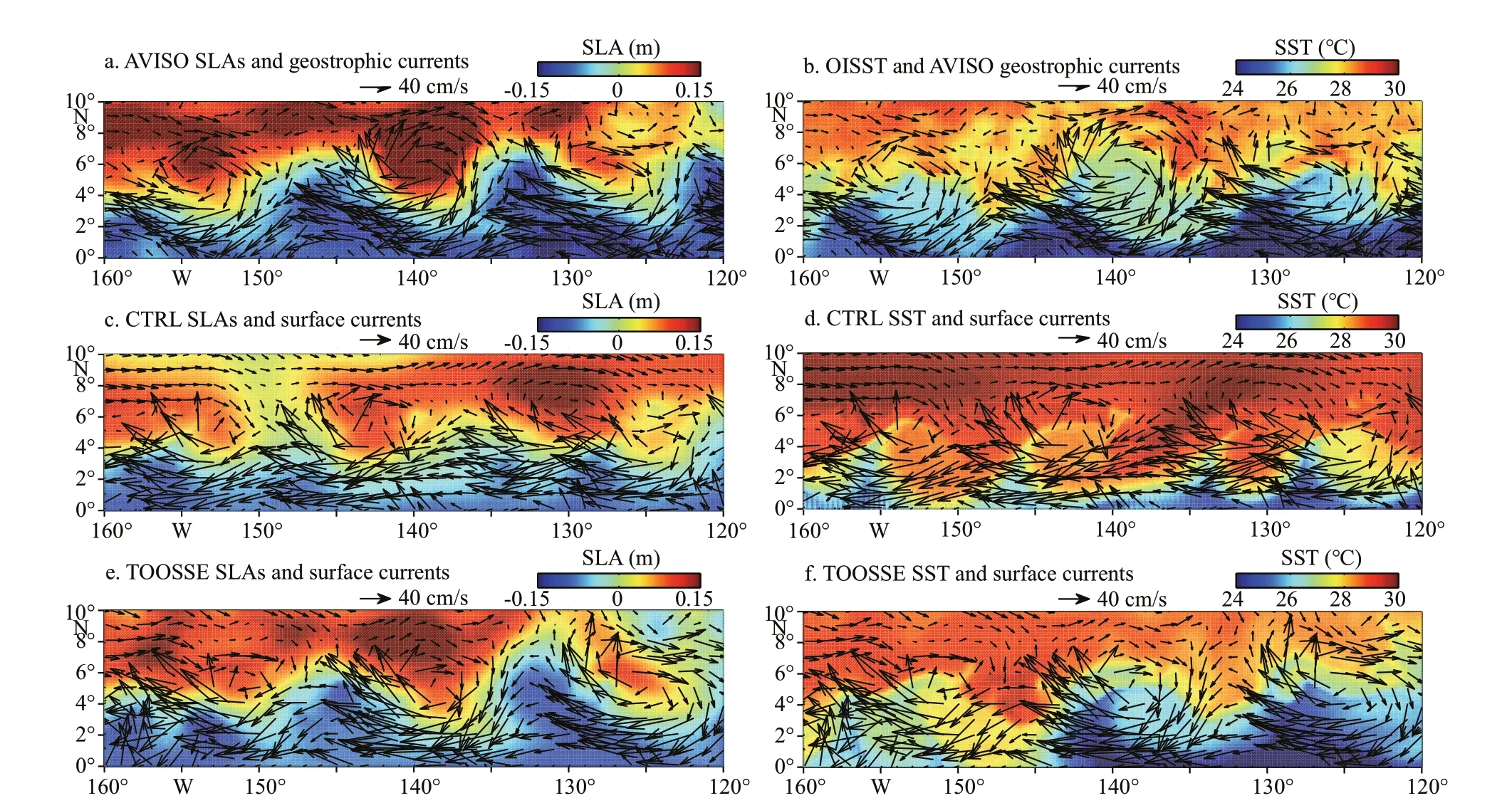
Fig.12 Daily TIW properties on Sep. 6, 2016

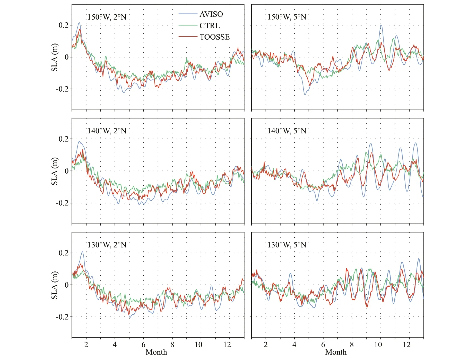
Fig.13 Time series of daily SLAs (in m) from the AVISO data (blue), CTRL (green), and TOOSSE (red) at key locations along 2°N (left column) and 5°N (right column) of the TIW region in 2016

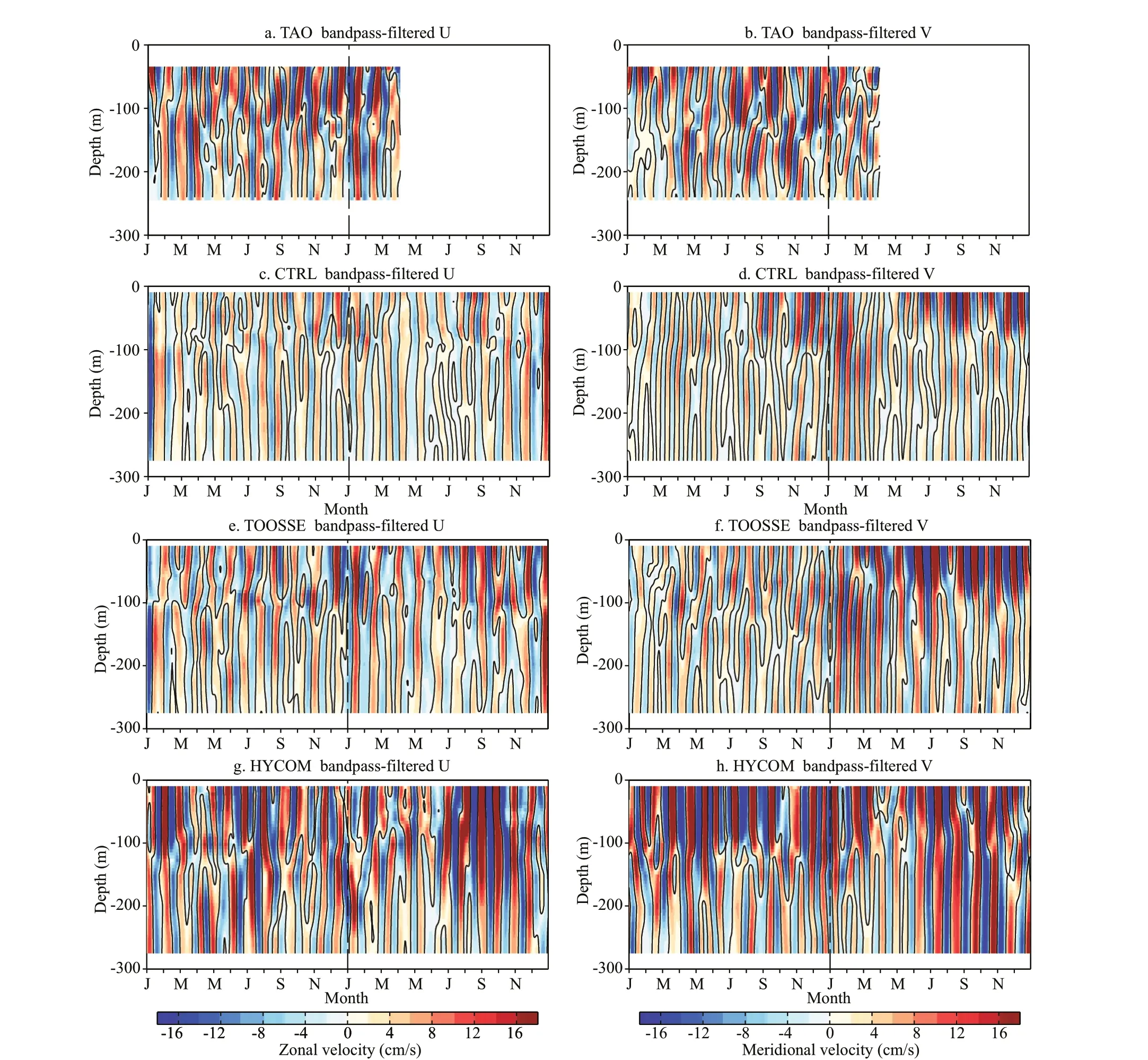
Fig.14 Time series of 15-40 days bandpass f iltered zonal (left column) and meridional (right column) velocities (in cm/s)at 140°W, 0°N (representing TIWs), from the mooring ADCP of TAO (a, b), the CTRL (c, d), TOOSSE (e, f), and HYCOM (g, h)

5 DISCUSSION AND SUMMARY

The low- to mid-latitude Pacif ic and Indian Oceans,along with the South China Sea and Indonesian archipelago in-between, play an essential role in the variability of global climate system, yet, large modeldata misf its remain in modern OGCMs. By using the 4D-Var (adjoint) methodology, we build an eddypermitting/resolving, dynamically consistent 4D ocean state estimate synthesis of the region over the years 2015 and 2016. This synthesis is named the Two Oceans One Sea state estimate (TOOSSE) and can better simulate the mean and time-varying state of the ocean than its unconstrainted control simulation.The misf its relative to observational constraints are reduced by over 40% in the SST, SSS, and the subsurface temperature and salinity, and by ～20% in mean SSH. The ocean state estimate is also largely consistent with a wide variety of independent observations, including TAO/TRITON, RAMA,OSCAR, and IOCAS. The large-scale pattern,mesoscale variability and seasonal to year-to-year (EI Niño to La Niña) variability are all well captured for the SLAs, temperature, and velocities (Section 4).

The adjustments of the air-sea f luxes in TOOSSE show multi-scale variations. Those of the zonal wind speed and heat f lux f ields are on both large and mesoscales, while those in precipitation are on basinscale. The adjustments of background vertical diff usivity exhibit a signif icant elevation in the thermocline around the equator and a slight enhancement around 600-m depth at 25°N-32°N,which are consistent with the observed high level of vertical mixing in those areas (Section 3). Note that the surface f luxes f ields do not dynamically evolve in the ocean model, thus the adjustments of these control variables are not necessarily improved at every grid and time. This is because some uncertainties in oceanic dynamics might be projected onto the surface f luxes f ields, and hence unphysical adjustments to surface f luxes could be induced. However, previous studies that focused on the adjustments to air-sea f luxes based on the ECCO/GECCO synthesis(Stammer et al., 2004; Romanova et al., 2010) suggest that both the time mean and the seasonal cycle of the estimated surface f luxes are in general agreement with that of other independent estimates. A detailed comparison between the adjustments to surface f luxes and independent data would be made later.

However, we note that there are still inconsistencies between TOOSSE and observations, particularly in SLAs. The cost function of SLAs reduces only by～10%, much less than for other contributors; the characteristic scale of SLAs seems larger of TOOSSE than that of AVISO poleward of 20°, though TOOSSE has a f iner resolution. A possible reason for the small cost function reduction could be that the mesoscale eddies in the mid latitudes are more nonlinear and unpredictable, so that the TOOSSE eddies cannot match the observations exactly in sizes, locations, and time. Using a much shorter assimilation window together with a less viscous adjoint model may have the potential to amend this problem (Verdy et al.,2017). The reason for the larger characteristic length scales than those of AVISO could be that TOOSSE at the same resolution reproduces fewer details than AVISO, because it requires a viscous part of the spectra from the diff usivity/viscosity for numerical stability so that some ability in producing f ine scale structures loses. Moreover, some recent ocean data assimilation studies suggested that the simulations of the SLAs, thermohaline structures, and equatorial currents can be improved by assimilating velocity prof iles (Liu et al., 2018, 2020), and this method might be adopted in the future development of the TOOSSE.

Nevertheless, as the f irst ECCO-based eddypermitting regional state estimate synthesis that connects the tropical Indian and Pacif ic oceans,TOOSSE is proved success in parameter optimization and ocean state estimate, which can provide accurate boundary conditions for regional ocean models within its domain. In addition, it produces many other important physical phenomena (e.g., the elevated mixing in equatorial thermocline, which may be essential for the local currents) that calls for a more detailed study.

6 DATA AVAILABILITY STATEMENT

All data generated and/or analyzed during this study are available from the corresponding author.

7 ACKNOWLEDGMENT

The simulation work was carried out at National Supercomputer Center in Tianjin, and the calculations were performed on TianHe-1A. We are grateful to two anonymous reviewers for their very helpful comments and recommendations.