A Fast Charging–Cooling Coupled Scheduling Method for a Liquid Cooling-Based Thermal Management System for Lithium-Ion Batteries

Siqi Chen,Nengsheng Bo,Akhil Grg,Xiongin Peng,Ling Go,*

a State Key Laboratory of Digital Manufacturing Equipment and Technology,School of Mechanical Science and Engineering,Huazhong University of Science and Technology,Wuhan 430074,China

b Intelligent Manufacturing Key Laboratory of Ministry of Education,Shantou University,Shantou 515063,China

ABSTRACT Efficient fast-charging technology is necessary for the extension of the driving range of electric vehicles.However,lithium-ion cells generate immense heat at high-current charging rates.In order to address this problem,an efficient fast charging–cooling scheduling method is urgently needed.In this study,a liquid cooling-based thermal management system equipped with mini-channels was designed for the fastcharging process of a lithium-ion battery module.A neural network-based regression model was proposed based on 81 sets of experimental data,which consisted of three sub-models and considered three outputs:maximum temperature,temperature standard deviation,and energy consumption.Each sub-model had a desirable testing accuracy(99.353%,97.332%,and 98.381%)after training.The regression model was employed to predict all three outputs among a full dataset,which combined different charging current rates(0.5C,1C,1.5C,2C,and 2.5C(1C=5 A))at three different charging stages,and a range of coolant rates(0.0006,0.0012,and 0.0018 kg·s-1).An optimal charging–cooling schedule was selected from the predicted dataset and was validated by the experiments.The results indicated that the battery module’s state of charge value increased by 0.5 after 15 min,with an energy consumption lower than 0.02 J.The maximum temperature and temperature standard deviation could be controlled within 33.35 and 0.8 °C,respectively.The approach described herein can be used by the electric vehicles industry in real fast-charging conditions.Moreover,optimal fast charging–cooling schedule can be predicted based on the experimental data obtained,that in turn,can significantly improve the efficiency of the charging process design as well as control energy consumption during cooling.

Keywords:Lithium-ion battery module Fast-charging Neural network regression Scheduling State of charge Energy consumption

1.Introduction

Owing to the significant challenges of fossil fuel shortages and greenhouse gas emissions,the global transportation industry is replacing traditional vehicles with clean energy automobiles[1].Rechargeable batteries are the central technology of electric vehicles(EVs),and lithium-ion battery cells are mainly used in energy storage devices for their many advantages:①high energy density,②high power density,③long cycle life,and ④low self-discharge rate.Lithium-ion battery cells are also widely used in various kinds of energy storage devices[2].However,despite its many advantages,a lithium-ion cell’s performance is sensitive to the ambient temperature.Previous research has shown that temperature strongly affects a lithium-ion battery cell’s charging/discharging efficiency,and this hinders the development of fast-charging technology.Severe temperatures accelerate the aging process,shorten the battery cells’lifetime,and can even result in thermal runaway.It is important to control the maximum temperature during the fast-charging process[2–4].Moreover,the uniformity of a battery module’s temperature distribution affects inconsistencies among the battery cells,which leads to the uneven rates of aging and a decay of the battery module’s lifespan.Considering the severe heat generated during the fast-charging process,it is vital to maintain the maximum temperature of a lithium-ion battery module within the range of 25–40 °C.Also,its temperature standard deviation(TSD)should be controlled at below 5 °C[5,6].

A battery thermal management system(BTMS)consists of a cooling function and a heating function.This study focuses on the cooling technology for the fast-charging process.Several kinds of cooling strategies have been developed for battery thermal management,such as air cooling,liquid cooling,a cooling method based on the phase change principle,and combinations of these.Air cooling,with its advantages of lower consumption and a simple structure,has become a commonly used method in EVs.Various studies have investigated this method before,through theoretical analysis and experimental validation,which were performed to enhance the cooling performance.These studies include flow channel structural design[7,8],battery cell layout design[9–11],and certain controlling methods of the BTMS[12].However,air cooling cannot provide sufficient cooling performance in several applications,especially under extreme high ambient temperatures or high charging/discharging current rates with insufficient heat conductivity of the coolant(air)[13].

Phase change materials(PCMs)are currently employed in cooling systems because they improve the uniformity of the battery module’s temperature distribution[14].However,PCMs cannot be widely employed in EVs because of their inadequate longterm cooling performance,which results from their intrinsic lower heat conductivity[15].Some recent studies were proposed to investigate PCM cooling efficiency under fast-charging.To enhance the heat conductivity,composite PCMs were studied by combining paraffin wax with aluminum,copper,graphite,graphene,or hexagonal boron nitride.However,the latent heat capacity of the PCMs decreased because of these combinations.Moreover,there is a significant volume consumption when PCM-based thermal management systems are used under fast-charging conditions.Under an 8C(1C=5 A)charging current rate,the volume consumption increases to 1.50–1.62 times that of traditional utilization[4,16,17].

Heat pipes have also been used in BTMS for their gas–liquid phase-changing characteristics[18].Rao et al.[19]studied the cooling performance of heat pipes in experiments.Their results indicate that the maximum temperature can be controlled within 50°C if a single cell’s heat-generating power is less than 50 W.Wu et al.[20]conducted a comparison between natural convection,forced convection,and heat pipe-cooling,and concluded that heat pipe-cooling is efficient in maintaining temperature rise.However,the effective thermal conduction area of traditional tubular heat pipes has the feature of ‘‘line contact” between the heat pipes’ evaporators and battery cells’ surface,which results in insufficient cooling performance and considerable TSD of the battery module[21].Zhao et al.[22]designed a flat plate-based heat pipe with mini-channels inside,which contacted well with prismatic battery cells,and it has become a candidate choice for cooling structures.

The advantages and disadvantages of various battery thermal management methods are compared in Table 1.Compared with the other cooling strategies,liquid cooling is a more efficient approach owing to its higher specific heat capacity and a uniform temperature distribution.However,liquid cooling-based thermal management systems can be error prone,and the assembly process and maintenance are much more complicated and expensive because the BTMS includes some additional equipment(pipes,pumps,or heat exchangers)[23].Moreover,the pressure drop between the inlet and outlet leads to unavoidable energy consumption[23].Furthermore,the battery cells of a battery module should be arranged under adiabatic conditions to avoid thermal runaway.Mei et al.[24]proposed three three-dimensional layered electrochemical–thermal models with various unit numbers.These were validated by experiments at various discharging current rates(0.5C,1C,1.5C,and 2C).The results indicated that a one-unit model needed a lower computational load,and this was helpful for the adiabatic studies.Previous studies on liquid cooling were conducted mainly on the structural design of flow channels[25–27]and on the enhancement of heat conduction by the coolingmedium[28–30].Chen et al.[31]proposed a comprehensive optimization design for a liquid cooling-based battery module and validated the design by experiments.The results indicated that the battery module’s thermal performance(maximum temperature and TSD)was significantly enhanced after the multi-objective structural optimization design.A liquid cooling-based BTMS was also verified to be effective in the discharging process of a lithium-ion battery module under a wide range of current rates.Panchal et al.[32]designed a liquid cooling plate for a lithium-ion battery module discharged at a 4C current rate.A cascade-based liquid cooling structure has been shown to have the ability to reduce a lithiumion battery module’s TSD from 7 to 2°C[33].

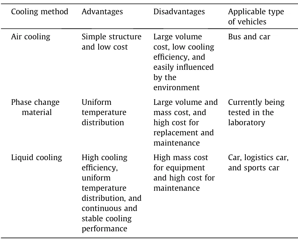
Table 1 Advantages and disadvantages of various battery thermal management methods.

Previous studies have revealed the superiority of liquid coolingbased battery modules.It has been shown that a battery module’s maximum temperature and TSD can be maintained within an appropriate range.However,these studies focused on the structural design of the thermal management system and on the thermal performance of liquid cooling-based battery modules under various working conditions.There is a lack of studies investigating a fast charging–cooling coupled scheduling which is necessary in order to enhance the driving range and charging efficiency.Moreover,in order to ensure driving safety and avoid overheating or an uneven temperature distribution,thermal management during the fast-charging process is also significant.There is a limited number of studies on combining fast-charging process scheduling with thermal management.The schedule selection reaches a reasonable tradeoff between the charging speed,cooling efficiency,and energy consumption that is applicable for EVs.

This study addressed the above issues through

(1)Designing a liquid cooling-based thermal management system equipped with mini-channels for the fast-charging process of a lithium-ion battery module;

(2)Proposing a neural network-based regression model in order to design an efficient fast charging–cooling coupled scheduling method;

(3)Employing the proposed regression model to predict three results from a full dataset,which combines a range of charging current rates(0.5C,1C,1.5C,2C,and 2.5C)at three different charging stages,and a range of coolant rates(0.0006,0.0012,and 0.0018 kg·s-1);

(4)Selecting an optimal fast charging–cooling coupled schedule from the predicted dataset by setting constraints;

(5)Validating the optimal schedule through the experiments.

2.Design of liquid cooling-based battery module

2.1.Cooling structure design for fast-charging

A liquid cooling-based battery module is shown in Fig.1.A kind of 5 A·h lithium-ion cell was selected,with its working voltage ranging from 3.20 to 3.65 V.Eight prismatic battery cells(considering the battery testing machine’s voltage limitation)were arranged on the top surface of a cooling plate.The heat generated from the battery cells was conducted and dissipated to the coolant flowing through the mini-channels,which resulted in a lower volume cost and provided sufficient thermal conductivity.The side surfaces between the single cells were separated by heatinsulating cotton designed to avoid the interaction between single cells under the effect of overheating.This structural design is accessible for EVs in real applications.

Aluminum alloy 7075 was selected for manufacturing of the cooling plate by milling,considering the high thermal conductivity and low cost of this material.Antifreeze was selected as the coolant,which consisted of ethylene glycol(50%)and water(50%).Antifreeze is commonly used in EVs and traditional vehicles for its lower ice point,especially in high-latitude areas.

2.2.Experimental configuration design

The experimental setup is shown in Fig.2.Eight single cells were connected in series,and the positive and negative electrodes of the module were connected to a battery testing machine(BTS-4000,Neware Electronics Co.,Ltd.,China).Four K-type thermocouples were attached to the same sidewall of each cell to measure the real-time temperature during the 15 min fast-charging process.A pressure sensor was attached to the inlet of the cooling plate;the real-time inlet pressure was also measured.The battery module’s temperature and pressure were recorded by two data loggers(THM001,Penghe Electronics Co.,Ltd.,China),with the values shown on the screens.A motor peristaltic tubing pump(Kamoer,China)was used to supply the coolant flow for the cooling system.The ambient temperature in the laboratory was set at 25 °C.The initial state of charge(SOC)value of the battery module was discharged to 0.2 before each set of experiments.

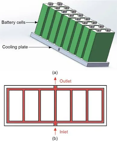
Fig.1.Schematic of the liquid cooling-based lithium-ion battery module.(a)Diagram of lithium-ion battery module;(b)diagram of mini-channel-based cooling plate.

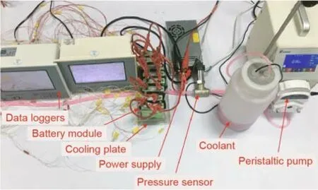
Fig.2.Image of the experimental setup.

3.Artificial neural network regression model

3.1.Artificial neural network regression

An artificial neural network is a kind of machine learning model employed for data classification or data prediction.The model structure is constructed based on data and learning rules[34].A neural network regression model is trained with data,based on a training algorithm,to predict a subsequent set of data.

As shown in Fig.3,an artificial neural network model consists of some nodes/neurons,which are set in multiple layers:an input layer,one or more hidden layers,and an output layer[34–36].Each node/neuron has an activation function,which calculates how much neuron is ‘‘stimulated.” At each layer,the collections of nodes/neurons transform the input parameters;these parameters are distributed to the next layer,which is described by Eqs.(1)–(3):

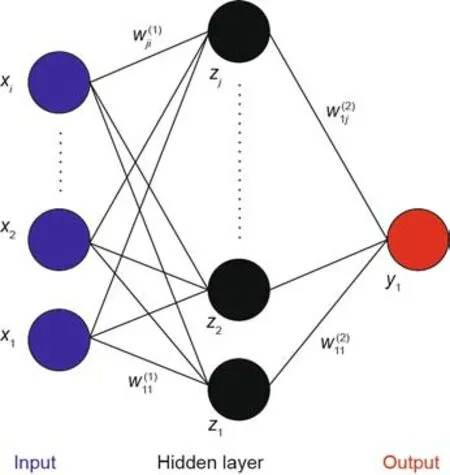
Fig.3.Diagram of neural network. x represents the input to the first layer; z represents the first layer’s output; y represents the output; i and j represent the neural network node index; xi represents the ith input to the input layer; zj represents the jth output of the first layer; wji(l) represents the weight between the jth node in the first layer and the ith node in the input layer.

wherexrepresents the input to the first layer;zrepresents the first layer’s output;iandjrepresent the neural network node index;nrepresents the index of the layer;represents the weight between thejth node in the first layer and theith node in the input layer;arepresents the input of the output layer;represents the output value ofith node in(n+ 1)th layer after being activated by the activation function;andwandw0represent the weight and bias between the neurons,respectively,which measures the significance of the data passed along the link(synapse).F(a)represents the activation function,which employs the hidden layer’s aggregated output to calculate the outputy[35,37].

The initial weights and biases are assigned randomly,and the training process continues until the desired output is obtained,which is evaluated by the cost function Eq.(4):

whereorepresents the desired output;E(w)represents the cost function evaluating the training process;wrepresents the weight;andkrepresents the index of the cost function calculation.The Levenberg–Marquardt(LM)algorithm is used in the neural network training process,which is a variation of gradient descent.The weight and bias of the neural network model are changed during the training process to minimize the error,which is described by Eq.(5):

where J=∂E/∂wrepresents the full-scale Jacobian matrix related tow,I represents the identity matrix,μ is combination coefficient,anderepresents the prediction error.

The LM algorithm starts with a forward computation by Eqs.(1)–(3).The prediction errors of the output layer and hidden layer are calculated by Eqs.(6)–(8):

where δ represents the prediction error of the output layer.

As shown in Eqs.(9)and(10),the Jacobian is calculated by a backpropagation process:

3.2.Configuration of neural network model

As shown in Fig.4,the entire charging process is divided into three stages;each stage lasts 5 min.I1,I2,andI3represent the charging current value at stages 1,2,and 3,respectively.Qrepresents the coolant flow rate of the fast-charging process.I1,I2,I3,andQare set as input parameters of the neural network models.

This study had three objectives:①maximum temperature(Tmax),② TSD,and ③ energy consumption(W)of the fastcharging process.These three parameters were set as output parameters of three neural network models(NN1,NN2,and NN3).

The value of the liquid cooling system’s energy consumption is calculated by Eq.(11):

Fig.4.Schematic of the three stages during the fast-charging process.

wherePrepresents the power consumption of the cooling system;trepresents time.

The TSD is calculated based on all of the measured temperature values from the temperature sensors and is described by Eq.(12):

whereTrrepresents the temperature value of each temperature sensor,represents the average temperature value of all the temperature sensors,andrrepresents the battery cell index.

All of the training data are from experiments and three charging current rates were selected for the three stages of the experimental charging process:①0.5C,②1.5C,and ③2.5C.Three coolant flow rates were also selected for the charging process:①36 mL·min-1,②72 mL·min-1,and ③108 mL·min-1.As shown in Fig.5,a total of 81 sets of experimental data were obtained for the training process.

The theoretical capacity is defined based on the assumption that all of the active substances in an electrode participate in the battery cells’ electrochemical reaction,which is treated as the highest theoretical value calculated according to Faraday’s law.In this study,the theoretical capacity of the battery cell is 5 A·h.The SOC value of the battery module is employed to evaluate the charging effect,which is calculated by Eq.(13):

whereIrepresents the charging current.

Specific information about the training dataset and corresponding SOC value is listed in Table 2.

Table 2 (continued)

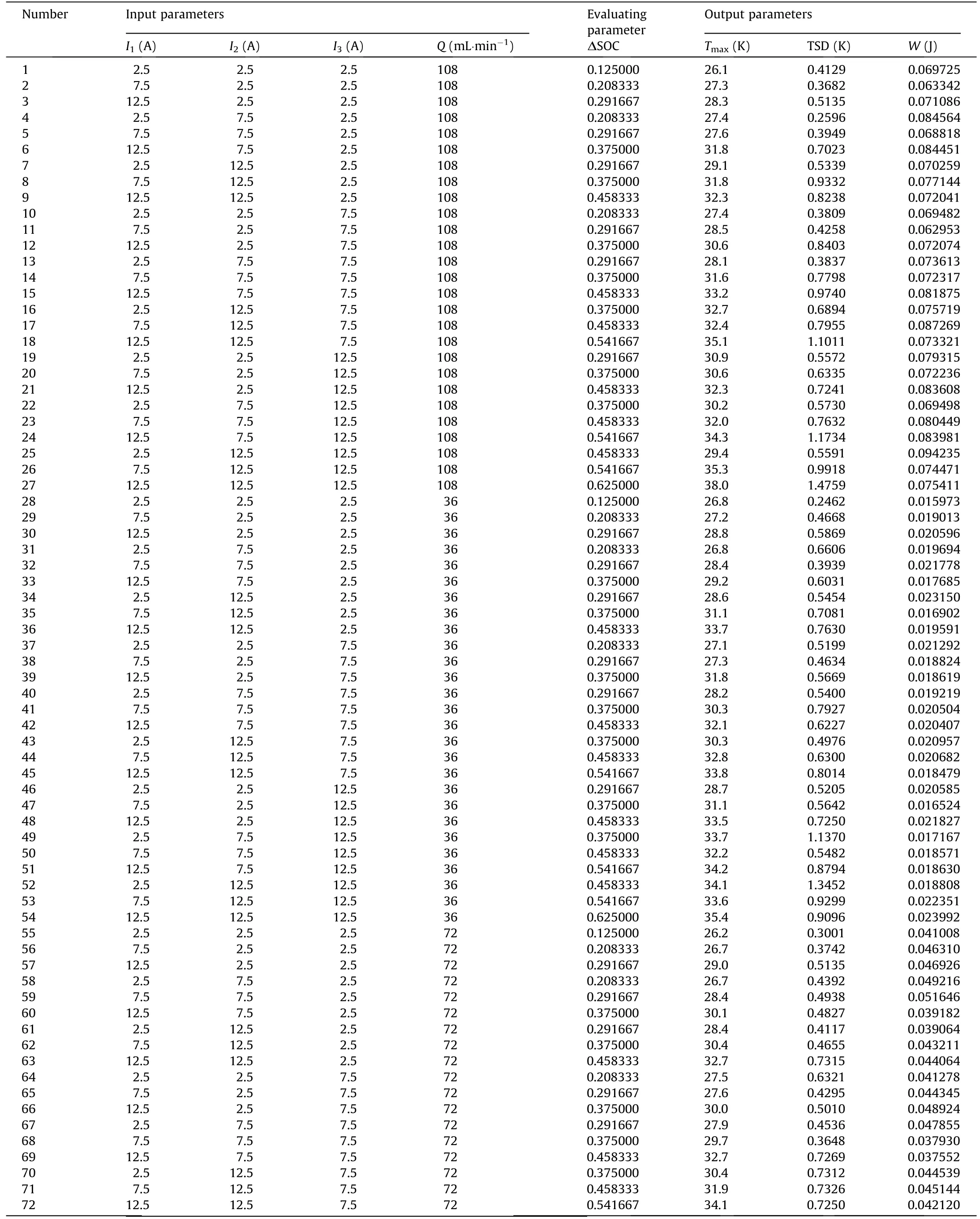
Table 2 Training dataset of the neural network model.

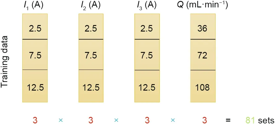
Fig.5.Composition of the experiment-based training dataset.

3.3.Structure of the neural network regression model

Unlike some battery cells’ behaviour-based governing equations,a neural network regression model is a ‘‘black box” model,which does not provide insight into how the hidden model’s structure actually works.Moreover,there are two problems for a nonlinear neural network regression model:① underfitting or overfitting,and ②the possible stagnation of the training process at the local optimal stage.

Some solutions are proposed to obtain a better regression performance:①input parameter preprocessing,so that representative ‘‘features” can be extracted from the data;②increasing the overall percentage of training datasets to cover the anticipated operational range;and ③ comprehensive cross-validation to enhance training performance when encountering an unknown usage profile[34].

The configurations of three neural network regression models are shown in Table 3.Each model consists of three layers,and these models are designed with the same activation function(a feedforward LM backpropagation approach)in the training process.As Fig.6 shows,the traditional neural network model is split into three sub-models,one for each objective(output parameter).Each input layer consists of the four input parameters(I1,I2,I3,andQ)and is followed by a hidden layer.The output parameter estimation responds to each of the input layers.The number of nodes in the input layer shows the exact number of input parameters used in the model.To obtain a continuous result,the hidden layers feed into another aggregation layer,which combines the results from the previous layers and feeds them to the output layer.To avoid overfitting and underfitting,two nodes/neurons in the hidden layer were implemented to get the desirable regression performance.Among the 81 sets of experimental data,a number of 73(90%)sets of experimental data were employed for training;four(5%)sets of experimental data were employed for validation;four(5%)sets of experimental data were employed for testing.One thousand epochs were set for the neural network regression training process.

Table 3 Configurations of three neural network regression models.

3.4.Regression performance evaluation of neural network model

As mentioned in Section 3.3,LM backpropagation was employed in order to enhance the model training rate related to pure error backpropagation or steepest descent,and this algorithm maintained the accuracy of the trained model.

The neural network regression model was trained with the designed model structure,input parameters,and number of nodes.The accuracy of both the training and the prediction/estimation was evaluated by the mean absolute error(MSE),which is expressed as Eq.(14).

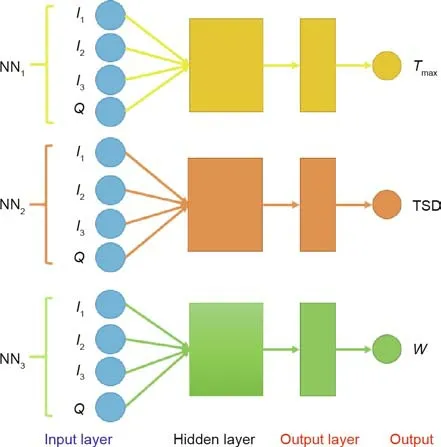
Fig.6.Diagram of the proposed neural network model.

whereeavgrepresents the average absolute error,Mrepresents the number of data points,Outputmrepresents themth estimated output parameter,and Outputr,mrepresents themth reference output parameter.The minimum error for the neural network estimation was found with the number of nodes per output parameter estimation layer set as two.

The training process of these three neural network models is shown in Fig.7.With the above neural network configuration,the estimation performance was improved,and the three regression models achieved a desirable speed of error convergence after initialization,during the training process.

As shown in Fig.8,high fitting accuracy rates were obtained after the training process.For the training process,the fitting accuracy rates of NN1,NN2,and NN3were 95.123%,82.866%,and 98.142%,respectively.For the testing process,the fitting accuracy rates of NN1,NN2,and NN3were 99.353%,97.332%,and 98.381%,respectively.The overall fitting accuracy rates of NN1,NN2,and NN3were 95.478%,83.496%,and 98.049%,respectively.All of the three neural network models achieved high accuracy rates,especially in testing;and the predicted values of the output parameters were close to the reference values.There was a slight difference between the measured and predicted energy consumption values,but the difference was within the tolerance limits.The results indicate that the relationship between the input parameters and output parameters was accurately modelled.With good regression performance of these three models,further prediction/estimation should be reliable.

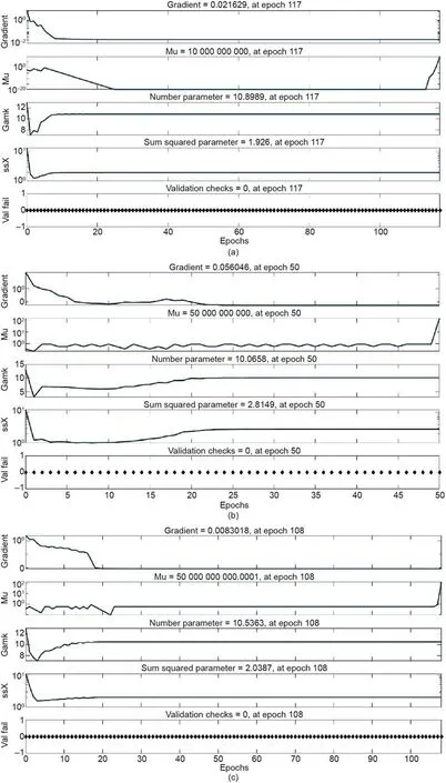
Fig.7.Training process of three neural network models.(a)Training process of NN1;(b)training process of NN2;(c)training process of NN3.Mu:reduction factor;Gamk:display frequency;ssX:inflation factor;Val fail:validation failure time.

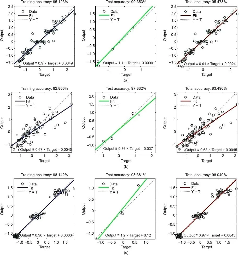
Fig.8.Regression performance of the three neural network models.(a)Regression performance of NN1;(b)regression performance of NN2;(c)regression performance of NN3.Y = T:trend line in ideal condition with 100% fitting rate;Y:output;T:target.

The error histogram plots of these three neural network models are shown in Fig.9.For the three neural network models,a number of 20 bins were distributed following the Gaussian distribution rules,which proved the representativeness of the training data.

4.Optimal charging–cooling schedule selection and experimental validation

4.1.Estimation of fast charging–cooling schedules based on the trained regression model

The trained neural network regression model was employed to estimate the results of some given input combinations.Some estimation results were compared with reference to some known experimental data to determine the accuracy and robustness of the trained model.

According to the current rates of fast-charging technology features,a total of five charging current rates were selected for the three stages of the charging process:①0.5C,②1C,③1.5C,④2C,and ⑤2.5C.Three coolant flow rates were also selected for the charging process:①36 mL·min-1,②72 mL·min-1,and③ 108 mL·min-1.Fig.10 shows the composition of the fast-charging designs.

There were 375 sets of fast charging–cooling schedules in a full dataset;and the maximum temperature,TSD,and energy consumption of these charging–cooling schedules were predicted using the proposed three neural network regression models(NN1,NN2,and NN3).Specific information and the SOC values of these fast charging–cooling schedules are listed as in Appendix A Table S1.

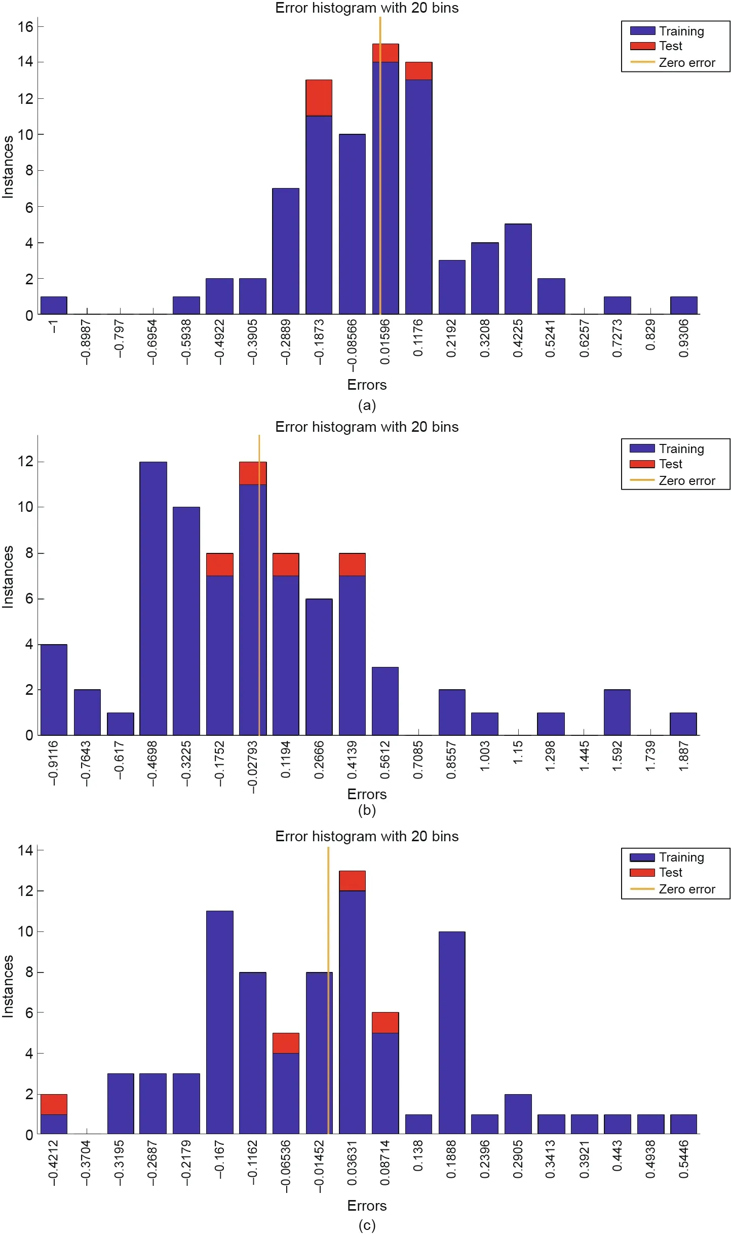
Fig.9.Error histogram of three neural network models.(a)Error histogram of NN1;(b)error histogram of NN2;(c)error histogram of NN3.Errors = Targets–Outputs.

4.2.Optimal charging–cooling schedule selection

To obtain an efficient fast-charging schedule,the thermal performance of the battery module should be controlled(maximum temperature and temperature distribution uniformity),the SOC value of the battery module must be charged to a high level within a short time,and the energy consumption of the cooling system should also be controlled.

In this study,the specific requirements for the optimal fast charging–cooling schedule are listed as follows:

(1)The SOC value of the battery module increases by 0.5 after the fast-charging process(15 min);

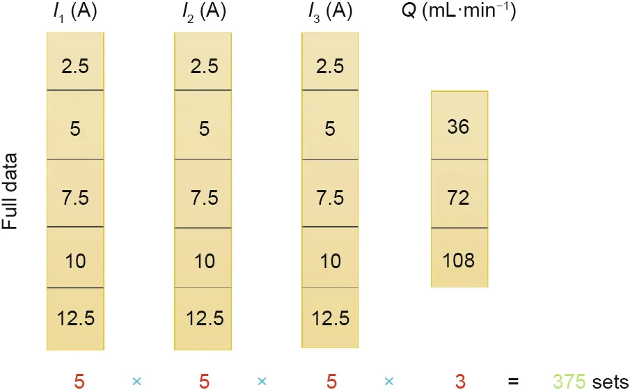
Fig.10.Composition of the fast-charging designs.

(2)The maximum temperature of the battery module should be lower than 306.5 K(33.35 °C);

(3)The TSD should be controlled within 0.8 °C;

(4)The energy consumption of the cooling system during the fast-charging process should be less than 0.02 J.

Addressing all of these constraints is essential for a comprehensive and reliable charging–cooling schedule design.The cooling effect,uniform temperature distribution,charging speed,and energy consumption should all be considered as having the same degree of importance.These selection standards are described by Eq.(15):

Schedule 50 was selected as the optimal fast charging–cooling schedule,and it was validated in the experiments using the above-described experimental setup.

4.3.Experimental validation

Figs.11 and 12 show the temperature and pressure curves of the fast charging–cooling design Schedule 50 in the experiments.

A comparison between the selected optimal fast charging–cooling schedule and the experimental data is presented in Table 4.

Table 4 Comparison between the selected optimal fast charging–cooling schedule and the experimental data.

As shown in the results,the differences between the predicted and experimental data are within the limits of tolerance.The deviation of maximum temperature,TSD,and the energy consumption of the cooling system are 0.468 °C,0.045327 °C,and 0.001694 J,respectively.This proves the prediction accuracy of the three proposed neural network regression models.Consequently,these models can be efficiently employed for fast charging–cooling coupled scheduling in real applications,with much lower costs.

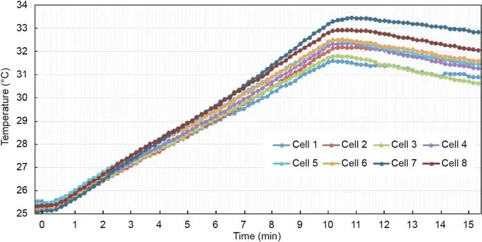
Fig.11.Temperature curve of the fast charging–cooling design Schedule 50.

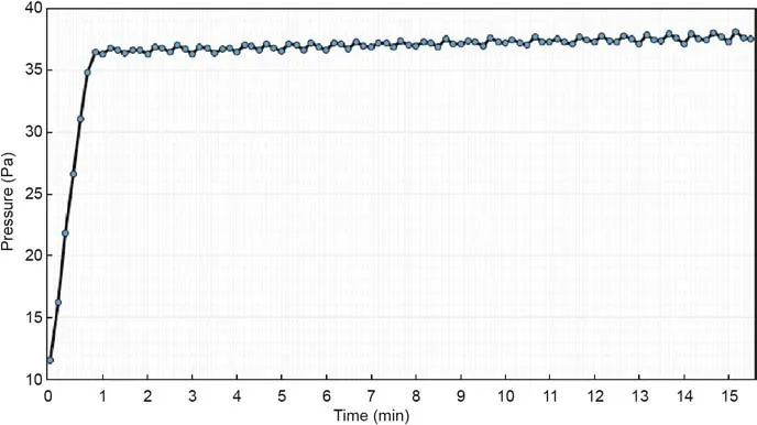
Fig.12.Pressure curve of the fast charging–cooling design Schedule 50.

5.Conclusions and further work

This study proposed a neural network-based regression model for fast charging–cooling coupled scheduling,which significantly saves time and cost during the fast charging-and-cooling design process.The proposed neural network model configurations achieve the desirable regression performance,and the designed configuration makes the estimation more realistic.The main conclusions of this study are listed below.

(1)The proposed model was trained based on 81 sets of experimental data,which consisted of three sub-models considering three targets:maximum temperature,TSD,and energy consumption of the cooling system.The regression results achieved high regression performance in tests,with 99.353%,97.332%,and 98.381% accuracy,respectively.

(2)The regression model was utilized to predict three target values for all of the combinations among a wide range of charging current rates(0.5C,1C,1.5C,2C,and 2.5C),at three different charging stages and a range of coolant rates(0.0006,0.0012,and 0.0018 kg·s-1).Moreover,an optimal fast charging–cooling coupled schedule was selected from the predicted dataset based on the constraints of the three targets.

(3)The optimal schedule was validated by experiments,and the results show that the battery module’s SOC value increased by 0.5 after 15 min of the fast-charging process.The energy consumption of this process was controlled within 0.02 J,and the maximum temperature and TSD were lower than 33.35 and 0.8°C,respectively.

The proposed method can be employed by the EVs industry in real fast-charging conditions,and the experimental test data can be used for regression training to predict the optimal fast charging–cooling schedule,which significantly promotes the efficiency of the charging process design and controls the energy consumption during the cooling process.

Further work will aim to develop and train neural network models to cover wider applications,and the effects of temperature changes in the environment and battery degradation may also be included.

Acknowledgements

This work was supported by the Program for Huazhong University of Science and Technology(HUST)Academic Frontier Youth Team(2017QYTD04),the Program for HUST Graduate Innovation and Entrepreneurship Fund(2019YGSCXCY037).Authors acknowledge Grant DMETKF2018019 by State Key Laboratory of Digital Manufacturing Equipment and Technology,Huazhong University of Science and Technology.This study was also financially supported by the Guangdong Science and Technology Project(2016B020240001),and the Guangdong Natural Science Foundation(2018A030310150).

Compliance with ethics guidelines

Siqi Chen,Nengsheng Bao,Akhil Garg,Xiongbin Peng,and Liang Gao declare that they have no conflict of interest or financial conflicts to disclose.

Appendix A.Supplementary data

Supplementary data to this article can be found online at https://doi.org/10.1016/j.ultsonch.2019.104640.