Physics-informed neural networks for estimating stress transfer mechanics in single lap joints#∗

Shivam SHARMA ,Rajneesh AWASTHI ,Yedlabala Sudhir SASTRY ,Pattabhi Ramaiah BUDARAPU

1School of Mechanical Sciences,Indian Institute of Technology,Bhubaneswar 752050,India

2Department of Aeronautical Engineering,Institute of Aeronautical Engineering,Hyderabad 500043,India

Abstract:With the explosive growth of computational resources and data generation,deep machine learning has been successfully employed in various applications.One important and emerging scientific application of deep learning involves solving differential equations.Here,physics-informed neural networks (PINNs) are developed to solve the differential equations associated with a specific scientific problem.As such,algorithms for solving the differential equations by embedding their initial and boundary conditions in the cost function of the artificial neural networks using algorithmic differentiation must also be developed.In this study,various PINNs are adopted to estimate the stresses in the tablets and the interphase of a single lap joint.The proposed model is represented by two fourth-order non-homogeneous coupled partial differential equations,with the axial stresses in the upper and lower tablets adopted as the dependent variables.The axial stresses are a function of the tablet length,which presents the independent variable.Therefore,the axial stresses in the tablets are estimated by solving the coupled partial differential equations when subjected to the boundary conditions,whereas the remaining stress components are expressed in terms of axial stresses.The results obtained using the developed methodology are validated using the results obtained via MAPLE software.

Key words:Physics-informed neural networks (PINNs);Algorithmic differentiation;Artificial neural networks;Loss function;Single lap joint

1 Introduction

The working mechanics of neural networks can be correlated with those of the human brain,which comprises billions of neurons.The concept behind artificial neural networks(ANNs)is to reduce a given task to the minimization of an objective function.The main advantage of ANNs is their capacity to efficiently perform parallel mathematical operations using high-level open source libraries such as Tensor-Flow,PyTorch,and Keras.This technique has been extended for solving numerous ordinary and partial differential equations(PDEs)(Yadav et al.,2015).In fact,the use of ANNs in conjunction with classical methods can lead to the development of efficient solution techniques for various physical problems involving PDEs.Meanwhile,physics-informed neural networks (PINNs) are neural networks trained to solve supervised learning tasks while satisfying the applicable laws of physics described by general nonlinear PDEs (Fang and Zhan,2020).These PINNs can replace the traditional discretization methods with a neural network that approximates the solutions of differential equations(Raissi et al.,2019;Kadeethum et al.,2020).A PINN algorithm for solving brittle fracture problems by minimizing the variational energy of the system is presented by Goswami et al.(2020),where the boundary conditions are entirely satisfied via appropriate modification of the neural network output.

In recent years,deep machine learning (DML)has been successfully applied in various fields,including academia (Waheed et al.,2020),financial markets(Yang et al.,2020),and nephrology(Thongprayoon et al.,2020).This is mainly due to the exponential growth of computational resources and data generation following significant scientific developments (Chen et al.,2014;Gupta et al.,2020).Samaniego et al.(2020) explored the area of deep neural networks for solving various PDEs in science and engineering,specifically in terms of mechanical problems based on the energy and natural loss function for a machine learning method.Meanwhile,a combined ANN/adaptive-collocation-strategy-based method for solving PDEs was introduced by Anitescu et al.(2019),where variable grid points are employed based on the value of the residual.Elsewhere,a deep collocation method using a feed-forward deep neural network to solve thin plate bending problems was proposed by Guo et al.(2019),and the applications of machine learning in composite materials modeling and design were reviewed by Chen and Gu (2019).An overview of machine learning applications in composite manufacturing was presented by Sacco et al.(2020),and a machine learning approach for predicting the effective elastic properties of composites with arbitrary shapes and inclusion distributions was proposed by Ye et al.(2019).Finally,a convolutional neural network model for predicting the mechanical properties of a 2D checkerboard composite with both soft and ductile and stiffand brittle phases was discussed by Abueidda et al.(2019).

Nacre is found in the inner layers of mollusk shells,enclosing the mollusk’s internal organs to protect the soft and delicate visceral mass (Budarapu et al.,2019).It consists of 95% brittle aragonite(calcium carbonate),with the remainder being organic polysaccharide arranged in form of brick and mortar structure (Barthelat et al.,2007).Such a combination of hard inclusions in a ductile matrix can sustain large deformations(Du et al.,2019;Magrini et al.,2019).The superior mechanical properties of nacre-like structures are because of the presence of a weak interface,which prevents the brittle failure of tablets under tension.In addition,smallsized tablets confer stronger and increased tensile strength compared with bulk aragonite.The underlying nano-mechanics governing the structural resilience and absorption of the mechanical energy of nacre is attributed to the nanoscale recovery of heavy deformation (Gim et al.,2019).Pan et al.(2017)proposed a thermally conductive polymer composite based on a bio-inspired naturally layered nacre-like brick and mortar structure.Moreover,Morsali et al.(2020)developed a combined statistical analysis and machine-learning-based computational approach to estimate the structure-property design strategies for nacre-like brick and mortar composites.The machine learning techniques were combined with specific tomography data to analyze the nacreous architecture in (Beliaev et al.,2020).The staggered arrangement of brick and mortar in nacre results in overlapping tablets connected by a polymer matrix,which can be further extended to develop optimized nacre-like materials with an optimum composition,microstructure,and size(Bertoldi et al.,2008;Barthelat,2014).

Lap joint configurations involve a multilayer structure comprising two substrates and an adhesive layer,with dissimilar geometric and material properties of the adherends that are common in various applications (Wang and Rose,2003).As a result of multiple layers with varying properties,the stress states prevailing at various levels in a bonded joint tend to be complex;therefore,considerable efforts have been devoted for developing accurate yet simple analytical methods for various types of lap joint,including double overlap,single lap,and single strap joints.Several valuable reports are available in the existing literature,including that from Adams and Mallick (1992).However,the accurate determination of the stresses at the critical locations within a joint requires detailed numerical computations using 3D elastic-plastic finite element analysis(Reinoso et al.,2019)or elaborate experimental techniques (Wang and Rose,2003).The temperature trends during friction-assisted joining as a function of different process parameters were investigated in(Lambiase et al.,2020)via the training,calibration,and validation of an ANN.A neural network and artificial intelligence (AI)-based model for studying the effects of welding parameters on the bead penetration area and predicting the bead penetration area for lap joints in the welding process was reported in(Oh et al.,2019).

An analytical model for predicting the interfacial shear and peel stresses in a double lap joint was discussed by Her and Chan (2019).Several experimental studies on adhesive-bonded carbon-fiberreinforced plastics (Budarapu et al.,2019;Gupta et al.,2019),joggled lap joints,and single lap joints are conducted in (Barile et al.,2020),with their attendant failure strengths reported.Rangaswamy et al.(2020) experimentally investigated the influence of overlap length,adhesive thickness,and adherend surface preparations on the failure behavior of adhesive-bonded joints using trained neural networks,whereas the failure load in single lap adhesive joints subjected to tensile loading was estimated using ANNs by Tosun and Çalık (2016).Gunes et al.(2011) employed ANNs and various genetic algorithms to study the influence of design parameters of the adhesive joint in their free vibration analysis (Budarapu et al.,2014) of an adhesively bonded functionally graded tubular single lap joint.Furthermore,the hygrothermal aging effect on the damage behavior of adhesive composite single lap joints was studied(Xu et al.,2019)using the acoustic emission technique in(Budarapu et al.,2015).

In this study,both the interfacial and normal stresses in a lap joint are estimated using a number of PINNs.A mathematical model for overlapping tablets joined by an adherend,which is represented by two fourth-order non-homogeneous coupled PDEs,is proposed,with the axial stresses in the upper and lower tablets adopted as the variables.As such,the axial stresses in tablets are estimated by solving the coupled PDEs when subjected to the boundary conditions,whereas the axial stress in the interphase is estimated by considering the force equilibrium.The remaining stress components,i.e.stresses along theydirection and shear stresses,are expressed in terms of axial stresses.The estimated stresses can be further used to estimate the fracture toughness of lap joints.The major features of the present study are as follows:

1.The creation of a novel PINN-based DML approach to solve two non-homogeneous coupled fourth-order PDEs.

2.The validation of the results obtained via the developed methodology using the results obtained via MAPLE software.

3.The inclusion of full Python script to estimate all the stress components in both the tablets and interphase.

2 Methodolgy

Machine learning involves the training of machines to learn from the data prior to its application for making logical decisions;this is achieved using appropriate algorithms.Furthermore,the decisionmaking capabilities,such as confirming the correctness of the estimated results,can be incorporated via DML,which involves employing the relevant neural networks and algorithms with the trained machines.Therefore,DML consists of some hidden/extra layers (up to 150) on top of the traditional neural networks,which generally contain 2–3 hidden layers.Deep learning is a subset of machine learning in AI that involves networks capable of unsupervised learning from unstructured or unlabeled data.In general,deep learning is employed to perform endto-end learning,where the network is given raw data and a specific task to perform.A key advantage of deep learning networks is that they generally continue to improve as the size of the data increases.

2.1 Physics-informed neural networks

A typical ANN operates like the biological(human) neural networks.Feed-forward neural networks are ANNs in which the connections between the units do not form a cycle.Here,the information flows only in a forward direction in the network without any loops,initially through the input nodes,followed by the hidden nodes,and finally through the output nodes.Feed-forward neural networks are primarily used for supervised learning where the data to be learned is neither sequential nor time-dependent;however,with the help of the universal approximation theorem,feed-forward neural networks can be used to compute a continuous real-value function.In general,an ANN consists of an input layer,generally a number of hidden layers,and an output layer (Fig.1).The hidden layers do not exist in a single-layer ANN;it presents a prototypicalmlayer ANN that computes a 1D output (OP) on ann-dimensional inputxxx={x1,x2,...,xn}.

For example,assuming that a feed-forward neural network is employed to compute a functionu(x;Θ) on a fixed-sized inputxandΘ,such that the network is set up by ˆuwith training pairs(x;Θ).Here,the derivatives of the networku(x;Θ)with respect to its inputxare estimated by applying the chain rule using algorithmic differentiation (AD),which is integrated in deep learning packages such as TensorFlow and PyTorch.In fact,AD is more efficient than the finite difference method,especially for input variables with a larger size compared with the dimensionality of the output variables.This is because the time complexity for reverse mode AD depends on the dimensionality of the output variables,whereas in the finite difference method,it depends on the dimensionality of the input variables.The training dataTin the problem domainΩwith a boundary indicated by∂Ωis divided into two sets,Tf∈ΩandTb∈∂Ω,and the loss function is defined as the weighted summation of theL2norm of error as follows:

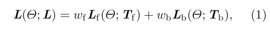
whereΘ={Wl,bl} contains the weight matrices and bias vectors of all the neurons in the neural networku,andwfandwbrepresent the weights of the points in the domain and on the boundary,respectively.Thus,after constructing the neural network and the suitable loss function,the objective is to estimate a good approximation forΘby minimizing the loss functionL.The loss function can be minimized using various gradient optimization techniques,such as the Adam and L-BFGS methods.However,the included Python script also contains commented commands to perform the optimization using the gradient descent optimizer.

Fig.1 shows a schematic of the PINN to solve the PDEs while considering the boundary and initial conditions,where the feed-forward neural network is highlighted in the neural network block.As the figure shows,an estimate of the stressesσ1andσ3was performed using the dimensions and material properties of the constituents of a lap joint.Furthermore,the derivatives of the stressesσ1andσ3were estimated via AD,which were subsequently used for the calculation of the loss function.The loss function was minimized through an iterative process to obtain the final values of the stressesσ1andσ3such that the boundary conditions were satisfied.

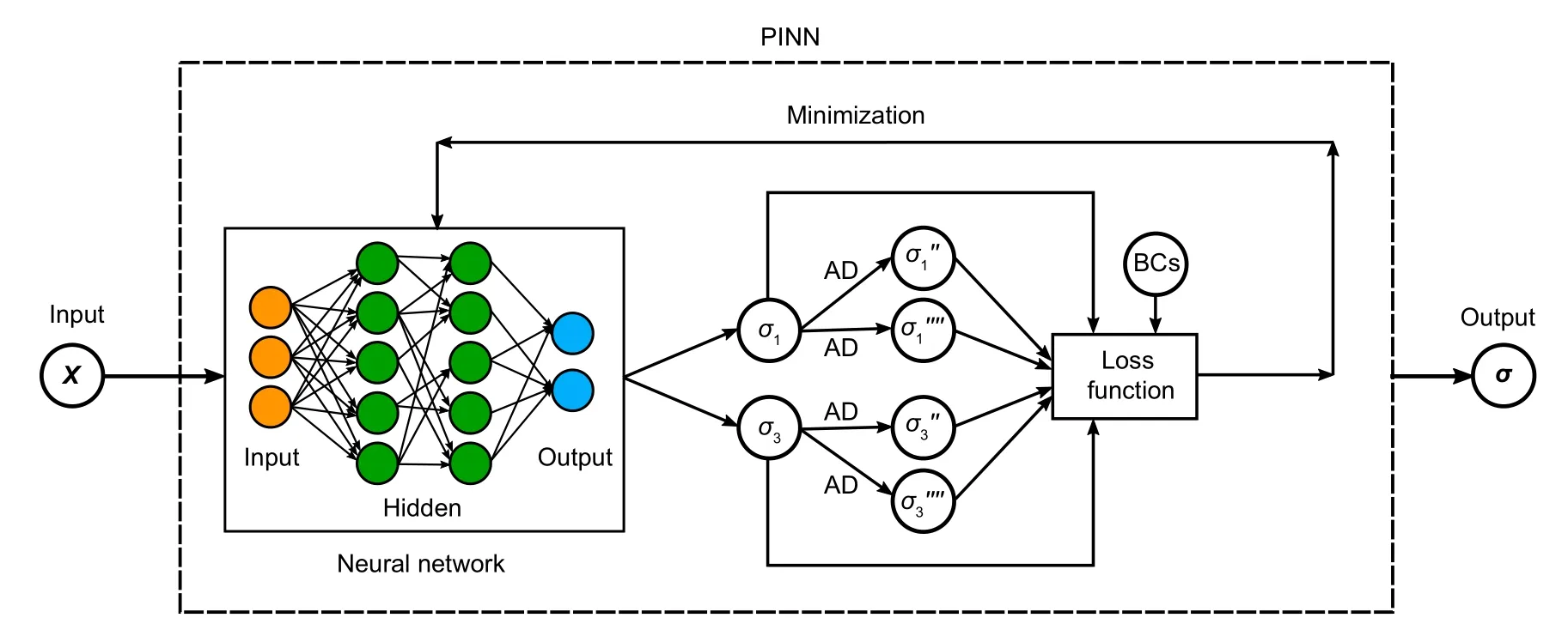
Fig.1 Schematic of the PINN to solve the PDEs while considering the boundary conditions (BCs) and initial conditions

3 Analysis of single lap joint

3.1 Analytical model of single lap joint

Considering a single lap joint,as shown in Fig.2,where two tablets with a lengthLand thicknessesh1andh2are bonded by a matrix with a lengthLand thicknessh.Here,the origin of the coordinate system is placed at the lower-left corner,and the distances of the top of the bottom tablet,matrix,and top tablet from the bottom surface are denoted byb,c,andd,respectively.When the right edge of the top tablet is subjected to a uniaxial tensile loadσ0,the reaction force on the left edge of the bottom tablet can be given byρσ0,whereρ=h1/h2.

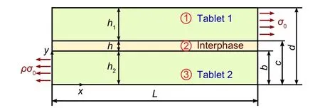
Fig.2 Schematic of two tablets with a length L and thicknesses h1 and h2 bonded by an interphase (matrix) with a length L and thickness h in the middle.An axial load σ0 was imposed on the right edge of the top tablet parallel to the tablet length,whereas the bottom tablet was fixed.The geometry was based on a nacre-like brick and mortar structure

Let the normal stresses along thexandydirections be denoted byand,respectively,and the shear stresses by,where the superscriptiindicates the constituenti=1,2,and 3,which represent the top tablet,matrix,and bottom tablet,respectively(Fig.2).Here the equilibrium equations along thexandydirections can be written as follows(Ajayan et al.,2003):

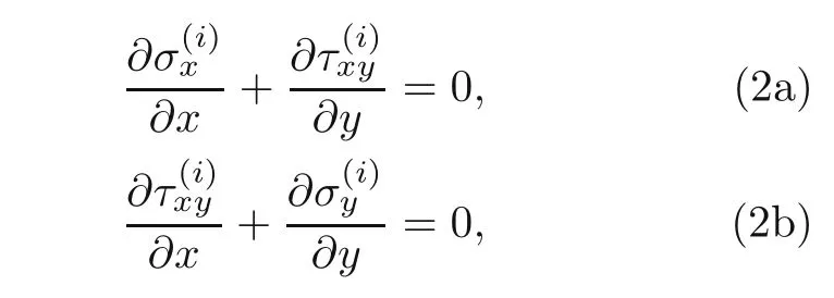
where the boundary conditions are given by:

Furthermore,considering the force equilibrium,σ2can be expressed in terms ofσ1andσ3as follows:

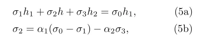
whereα1=h1/handα2=h2/h.The axial stressesσ1andσ3were estimated by minimizing the system potential energy,which can be expressed as

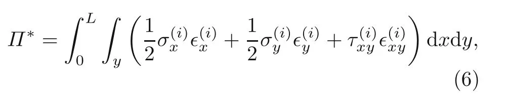
where∊xand∊yindicate the normal strains along thexandydirections,respectively,and∊xyrepresents the shear strain in thexyplane.The properties of the tablet and interphase used in this study are presented in Table 1.

Table 1 Material properties of the tablets and the interphase of the single lap joint (Fig.2) used in this study(Jackson et al.,1988;Barthelat and Espinosa,2007;Espinosa et al.,2009;Ni et al.,2015)

Therefore,considering the stress components in each of the constituents and the material properties presented in Table 1,the potential energy of the system can be estimated using Eq.(6).The estimated system potential energy was further minimized using the Euler-Lagrange variation principles,which resulted in the following simultaneous equations related to the axial stressesσ1andσ3in tablets 1 and 2,respectively:

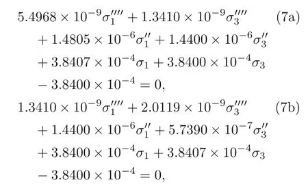
whereσ1andσ3are the axial stresses in tablets 1 and 2,respectively,and the length of the tablets(L) is considered to be 8 µm.The next objective was to solve the coupled partial differential equations(Eq.(7)) using neural networks for estimating the stressesσ1(x) andσ3(x),wherexis the length of the tablet defined in the domain 0≤x ≤L.The main steps in the solution algorithm of the developed PINN are summarized below.

1.Construct a neural network with two output variablesσ1,σ3=NN(x;Θ),whereΘindicates the parameters of the neural network,i.e.Θ={Wl,bl}is the set of all the weight matrices and bias vectors of the neural network,where 1≤l ≤nlandnldenotes the number of layers.

2.Prepare a training setNffor training the above constructed neural network.Each point in the training set lies within the specified domain of the differential equations.

3.Estimate the loss function by calculating the averageL2norm of the differential equations and the boundary conditions over the whole training set.The loss function is given by the following:

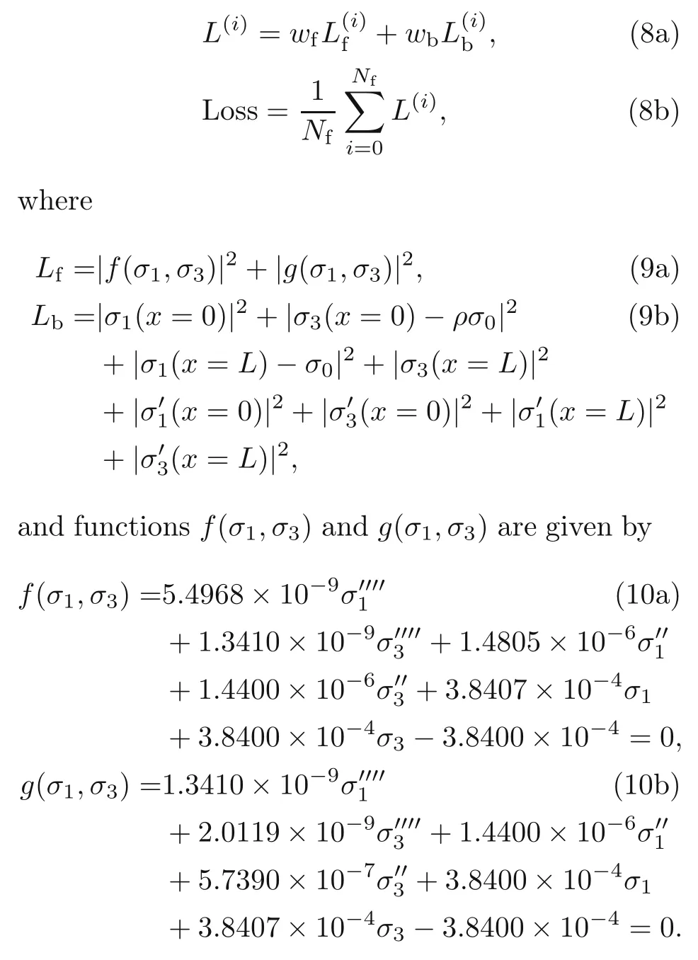
The derivative of the output variablesσ1andσ3of the neural network with respect to the inputxwas calculated by applying the chain rule of differentiation using AD,an inbuilt function of the TensorFlow deep learning framework.The loss function was prepared in such a way that the output of the neural network satisfied the differential equations as well as the imposed boundary conditions for all the points in the training set.

4.Optimize the loss function in Eq.(8) using the Adam and L-BFGS gradient-based optimization solvers to determine the optimal parameterΘ∗for the proposed neural network.

3.2 Implementation aspects of the neural network schema

The neural network was implemented using Python language version 3.6.9 in TensorFlow framework version 1.15.2;the developed neural network was trained using a Tesla T4 GPU card in Google Colab.An iterative process was followed in this study to ensure that the architecture of the neural network reached the least value of the loss function.A fully connected feed-forward artificial neural network architecture with three hidden layers (each layer contained 500 neurons),one input layer,and one output layer containing two output neurons was selected for the analysis.The network was comprehensively tested with varying number of neurons in each layer to test the convergence and repeatability of the results;the developed network produced stable results every time.The histograms formed during the network training are presented in Section S2 of the electronic supplementary materials(ESM),and the network architecture in the Python script is described in Listing S1 in the ESM.The implementation of the developed PINN is described in Listing S2 in the ESM.

The training data was obtained using Latin hypercube sampling(LHS),where the size of the training data set generated (i.e.Nf[training data]) was 5000.One-dimensional LHS involves dividing the cumulative density function intonequal partitions and then choosing a random data point in each partition.This type of sampling significantly reduces the number of iterations required to achieve a reasonable and accurate result.In fact,well-performed LHS can reduce the processing time by up to 50%;on the contrary,the LHS can lead to more accurate results when there is no time constraint.The training data sets in the Python script are described in Listing S3 in the ESM.

The initialization of the network using the correct weights can result in quick convergence with stable network loss function for a large number of iterations (hundreds of thousands).Therefore,the initialization step is critical to the model’s ultimate performance.In this study,we used the Xavier initialization function for the initialization of the neural network,i.e.initialization of the weights and biases.Xavier initialization involves controlling the constant variance across every layer,with the output centered around 0,indicating that the mean is 0.The variance of weights in layerlis given by the following equation:

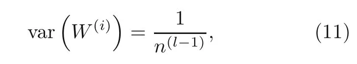
wheren(l−1)represents the number of neurons in the previous layer.The initialization steps in the Python script are presented in Listing S4 in the ESM.The initial parameters were set based on previous experience,which will be fine-tuned later.

Meanwhile,activation functions were incorporated in the neural network to introduce nonlinearity.These functions are generally employed to convert an input signal of a node in an ANN to an output signal,and the converted output signal is further used as an input to the next layer in the stack.In this study,the hyperbolic tangent activation function(Tanh)was employed as the activation function.However,the included Python script also contains commented commands to estimate the activation function using Sigmoid and rectified linear unit (ReLU) functions.The neural network parameters were optimized based on the loss function.As such,the objective was to minimize the loss for a given neural network by optimizing its parameters(weights and biases).In this study,we adopted a mean square error loss function,which is the square of the difference between the predicted value and that obtained via the neural network considering the boundary conditions and the predicted output based on the training values.The estimation of the loss function using the Python script is described in Listing S5 in the ESM.

Optimization algorithms were subsequently adopted to optimize the objective function,i.e.the loss function.Here,the mean square error loss function,as described above,was employed.When the loss function was close to zero,the solution could be deemed to be converging.The computer implementation program,developed in TensorFlow using Python script,for estimating the loss function and thus the stresses,is attached in the ESM.

3.3 Results and discussion

The series of differential equations developed in Section 3.1 was solved using the neural network model proposed in Section 3.2.Two different types of activation functions,the hyperbolic tangent (Tanh)and ReLU functions,were tested using the neural network architecture,with the results subsequently compared.Here,the results obtained via the ReLU activation function clearly required less computational time for each epoch compared with the Tanh activation function.This was evident given the number of epochs trained in the same time period for both the activation functions.However,the results estimated using the Tanh activation function were found to be more reliable and stable and were thus adopted for the subsequent analysis.This was because the Tanh activation function provided both positive and negative values,thus yielding more accurate results.

The variation in loss function while training the proposed PINN as a function of the number of iterations is plotted in Fig.3.As the figure shows,initially,the variation was slightly irregular before it smoothly decreased to approach zero according to the number of training epochs of the model.A combination of L-BFGS-B and Adam optimizers was employed here,with the specified iterations equal to 200.However,the error tolerance for the loss function was set to machine accuracy,which is of the order of 10−12.Therefore,beyond 200 iterations,the system would switch to the Adam optimizer until the specified error tolerance was achieved.However,the maximum number of iterations under any conditions should not exceed 50 000.

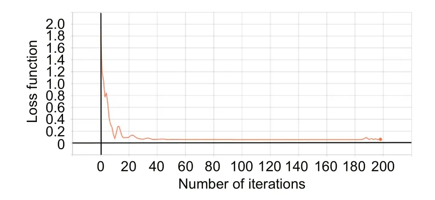
Fig.3 Variation in loss function during the training of the PINN with a number of iterations

A uniaxial loadσ0of 100 MPa was applied on the upper tablet parallel to its length while keeping the lower tablet fixed (Fig.2).The axial stresses in tablets 1 and 2,indicated byσ1andσ3,respectively,were estimated by minimizing the loss function(Eq.(8)) while being subjected to the boundary conditions described in Eq.(3).The distribution of the various stresses in tablets 1 and 2 and the interphase were plotted,as shown in Figs.4–6,where all the stresses were extracted at the mid-layer.Meanwhile,the variations in the axial stresses along the length of tablets 1 and 3 and the interphase were plotted,as shown in Figs.4a and 4b,respectively.Here,the axial stressesσ1andσ3clearly complemented each other,thus satisfying the boundary conditions.

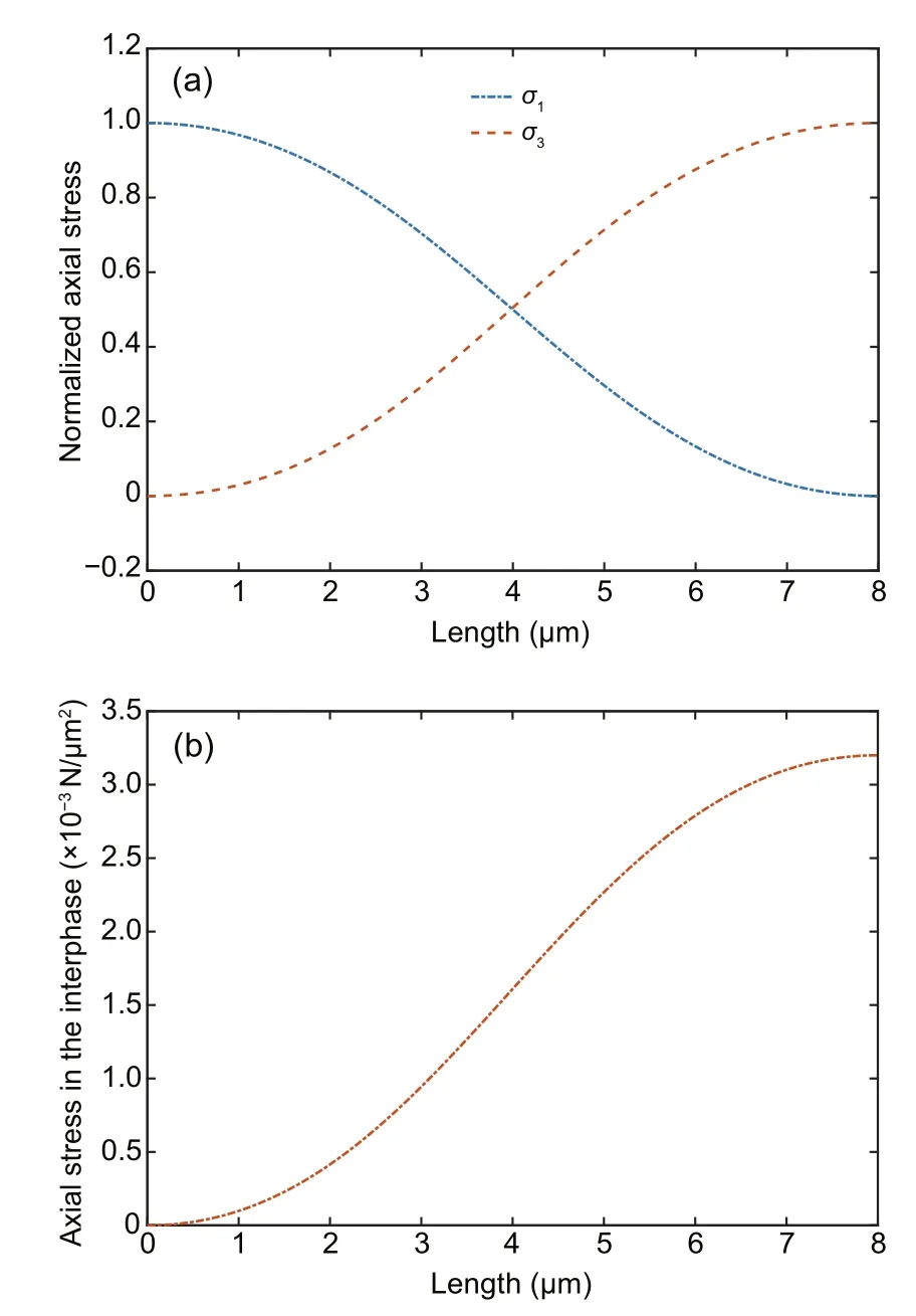
Fig.4 Distributions of the axial stresses in tablets 1 and 2 (a) and the interphase (b) as a function of tablet length

The variation in the shear stress in the interphase as a function of the length of the lap joint was plotted,as shown in Fig.5a.To verify the results obtained using the proposed model,the exact solution was estimated by solving the analytical model discussed in Section 3.1 using MAPLE software.A comparison of the interfacial shear stress estimated using the proposed method and the exact solution is shown in Fig.5a.Here,the exact solution was found to represent the physical phenomena,where the shear stresses at the edges were maximized over a small region and dropped down toward the center.However,as Fig.5a shows,the results based on the DML approach clearly represented the physical behavior,but they were not in close agreement with the exact solution.Specifically,the proposed DML approach was unable to capture the physical behavior at the interphase edges,which is a prevailing issue with DML-based approaches.This was further confirmed by the comparison of the normal stresses along theydirection in the interphase,as shown in Fig.5b,where the solution estimated using the developed DML approach clearly failed at the interphase edges (in the close-up regions).The normalized(with respect to the exact solution)error(difference of DML and exact solutions)in the shear stress estimated at the middle of the joint length was estimated to be 1.22%,and the average normalized error in the normal stress along theydirection in the interphase,calculated as the average of the normalized errors estimated at several points along the interphase length,was 26.19%.The estimated results and errors using the present DML approach are promising;however,advanced mathematical tools can be adopted to minimize the cost function with reduced errors.

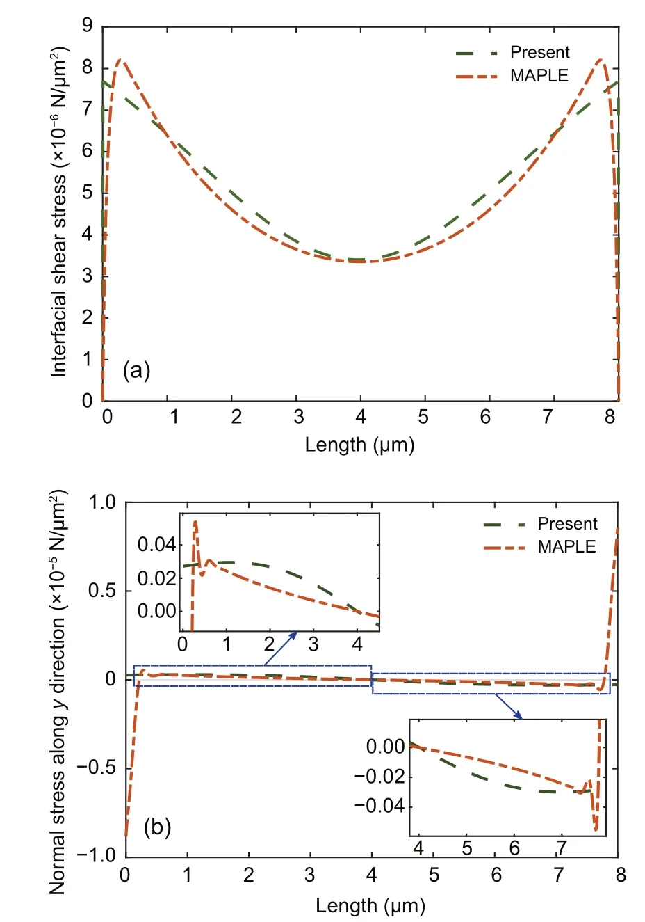
Fig.5 Distributions of the shear stresses () (a)and the normal stresses along the y direction ()(b) in the interphase along its length.The results estimated using the developed methodology were compared with those calculated using MAPLE software.Close-ups of the regions on the left and right sides around the center of the interphase are also shown

The distributions of the normal stresses along theydirection and the shear stresses in tablets 1 and 2 are shown in Figs.6a and 6b,respectively.

The normal and shear stresses in tablet 2 were significantly lower than those of tablet 1,mainly because the load was applied at the right edge of tablet 1 along the axial direction,i.e.the load was shear transferred to tablet 2 through the interphase.Hence,a part of the applied load was dissipated in the interphase in the form of shear and peel stresses.

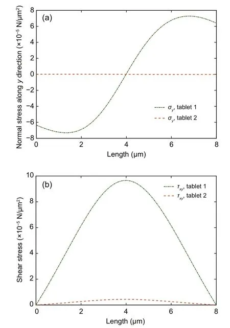
Fig.6 Distributions of the normal stresses along the y direction (a) and the shear stresses (b) in tablets 1 and 2

4 Conclusions

The mechanics of a single lap joint were investigated by solving a DML-based PINN.A uniaxial loading parallel to the tablet length was applied on the right edge of the upper tablet while keeping the lower tablet fixed.The developed framework was then extended to estimate the various stress components in a number of tablets as well as the interphase by solving the coupled fourth-order non-homogeneous PDEs equations subjected to the boundary conditions.The results obtained via the DML-based approach were then compared with the exact solution obtained using MAPLE software.

The interfacial shear stress estimated using the proposed method and the exact solution were also compared.Here,the results obtained via the DMLbased approach represented the physical behavior,although they were not in agreement with the exact solution.Specifically,the proposed DML-based approach was unable to capture the physical behavior at the interphase edges.Similar behavior was observed during the comparison of the normal stresses along theydirection in the interphase.The normalized error in the interfacial shear stress estimated at the middle of the joint length was found to be 1.22%,whereas,the average normalized error in the normal stress along theydirection in the interphase was 26.19%.

The method of using deep learning to solve the differential equations is a promising approach because the attendant computer codes are robust enough to handle the changes in the differential equations.Furthermore,the developed deep learning methodology can be used to solve complex equations or a system of equations(e.g.engineered interphases with a tailored elastic modulus).An iterative approach was employed in this paper to determine the correct hyper-parameters,which is essential for obtaining accurate results.Though the training of the neural network requires a computationally expensive approach,we believe that this method will continue to evolve with time,overcoming the above limitations,and it will be used to assist in solving various practical problems in future.

Contributors

Pattabhi Ramaiah BUDARAPU formulated the analytical model and designed the research.Shivam SHARMA developed the DML codes,processed the corresponding data,and wrote the first draft of the manuscript.Rajneesh AWASTHI,Yedlabala Sudhir SASTRY,and Pattabhi Ramaiah BUDARAPU revised and edited the final version.

Conflict of interest

Shivam SHARMA,Rajneesh AWASTHI,Yedlabala Sudhir SASTRY,and Pattabhi Ramaiah BUDARAPU declare that they have no conflict of interest.