A deep neural network-based algorithm for solving structural optimization#∗

Dung Nguyen KIEN ,Xiaoying ZHUANG,2,3

1Department of Geotechnical Engineering,College of Civil Engineering,Tongji University,Shanghai 200092,China

2Institute of Photonics,Department of Mathematics and Physics,Leibniz University Hannover,D-30167 Hannover,Germany

3Hannover Center for Optical Technologies,Leibniz University Hannover,D-30167 Hannover,Germany

Abstract:We propose the deep Lagrange method (DLM),which is a new optimization method,in this study.It is based on a deep neural network to solve optimization problems.The method takes the advantage of deep learning artificial neural networks to find the optimal values of the optimization function instead of solving optimization problems by calculating sensitivity analysis.The DLM method is non-linear and could potentially deal with nonlinear optimization problems.Several test cases on sizing optimization and shape optimization are performed,and their results are then compared with analytical and numerical solutions.

Key words:Structural optimization;Deep learning;Artificial neural networks;Sensitivity analysis

1 Introduction

Optimization is a significant tool in physical system analysis and decision science (Nocedal and Wright,2006).The motivation of optimization is using the limited resource to obtain the maximized utility(Kirsch,1993).There are three types of structural optimization problems,that is,sizing optimization,shape optimization,and topology optimization(Christensen and Klarbring,2009).In sizing optimization,the thickness of the structure type (e.g.cross-section area) is minimized.The contour or form of some specific parts of the structural domain boundary are of interest in shape optimization,whereas the entire material layout is minimized in topology optimization.A variety of methods have been devised to solve the optimization problems including the Newton method,quasi-Newton method,Gauss-Newton method(Nocedal and Wright,2006),and metaheuristic optimization algorithms (particle swarm optimization(Hu and Eberhart,2002),differential evolution (Storn and Price,1997),and some others (Kaveh,2017)).Exact optimization does not guarantee global minimum of the solution.Moreover,some metaheuristic optimization algorithms have the potential to detect it.

Several efficient methods could solve the nested formulation obtaining an explicit approximation in structural optimization(Christensen and Klarbring,2009),such as sequential linear programming(SLP)(Fletcher and Maza,1989) or sequential quadratic programming or convex linearization (CONLIN)(Fleury and Braibant,1986).SLP requires firstorder approximation and could be applied to solve a large range of structural optimization problems(Schittkowski et al.,1994).Recently,a multipoint exponential approximation(MPEA) has been introduced,which approves to be a good alternative(Canfield,2018).A strong competitor with better convergence properties is the method of moving asymptotes (MMA) (Svanberg,1987,2002).Level setbased optimization as presented in Ghasemi et al.(2017,2018) is another option.However,all these approaches require a sensitivity analysis,which is not always easy to carry out analytically.

Machine learning is an alternative to classical optimization approaches.Artificial neural networks(ANNs) are inspired by the animal brain.They can learn the performance tasks without being programmed (Goodfellow et al.,2016).ANNs to structural optimization problems were applied by Hajela and Berke (1991),Papadrakakis et al.(1998),and Papadrakakis and Lagaros(2002).Furthermore,the authors applied the backpropagation algorithm,which is among the most fundamental neural network architectures,and used a feedforward neural network.Recently,neural networks have also been applied to solve directly the underlying boundary value problem.Anitescu et al.(2019) trained the network at discrete collocation points.They considered not only the forward problem but also the inverse problem,which is similar to an optimization approach;in fact,it is more challenging to solve.Deep energy methods are an alternative to such collocation approaches as proposed by Goswami et al.(2020a,2020b),Nguyen-Thanh et al.(2020),and Samaniego et al.(2020).

We present a so-called deep Lagrange method(DLM)applied to sizing optimization and shape optimization inspired by the aforementioned methods.The method is based on the Lagrange duality and deep learning.The Lagrange duality theory provides a way to solve the original constrained optimization problem by looking at the dual problem (Boyd and Vandenberghe,2004).The input data are used in a deep neural network for training the neural network until the output values resemble closely the predicted values.Minimum input values will be found when the min-max problem in Lagrange duality is solved following the interpolation from deep learning.Therefore,this deep learning-based method is an improvement when avoiding sensitivity analysis.It employs a large number of input data for the neural network.However,the proposed method is potentially applied to structural optimization problems that require a small number of design variables.

2 Deep Lagrange method

2.1 Lagrange duality approach

Methods based on Lagrange duality require the reformulation of the nested formulation optimization problem into the Lagrange duality formulation.Christensen and Klarbring(2009)provided a general optimization problem with inequality constraints.

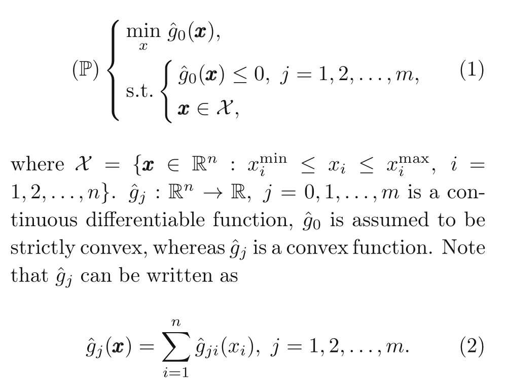
Then,the Lagrangian functionLof optimization problem(P)reads

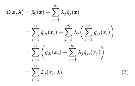
where Lagrange multipliersλj ≥0,j=1,2,...,m.The Lagrange dual problem can be formulated as

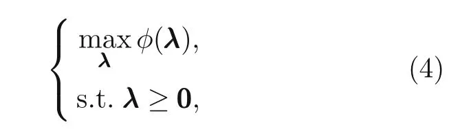
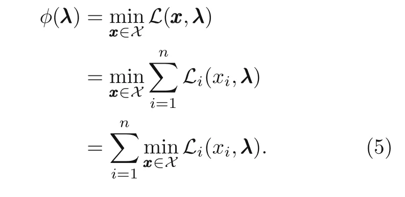
with the dual objective function given by

2.2 Deep Lagrange method for optimization problems

2.2.1 Neural network architecture

The feed forward neural network architecture is shown in Fig.1.The first layer (0th layer) is the input layer,whereas the last layer(Kth layer)is the output layer.The layers in between are the hidden layers.Each layer contains a certain number of nodes and is connected with the next layer.

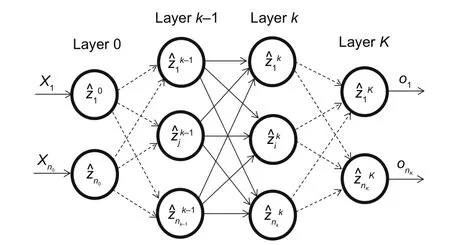
Fig.1 A feedforward deep neural network with K layers

The input vector is denoted byXXX,andooo=(X1,X2,...,Xn0) the output vector.Fig.2 shows the connection of the nodes between the layers.Each node connects the next layer through weightswwwand biasbbb.

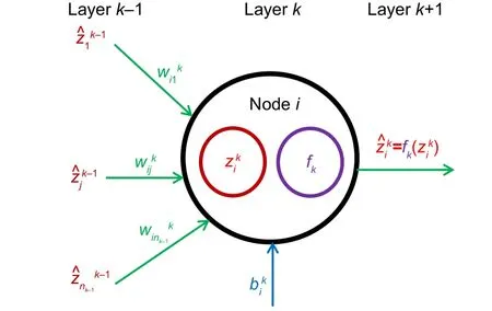
Fig.2 Output calculation at the ith node in the kth layer

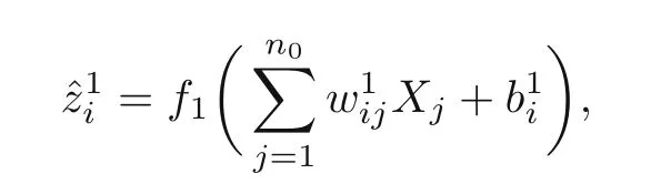
The activation function,fk,evaluates the value of theith node in the hiddenkth layer at each node in the hidden layer.The output of the nodes is calculated as(Fig.2)

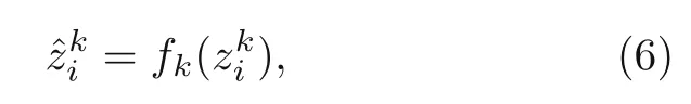
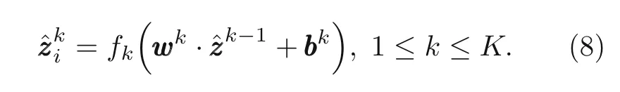
also written as

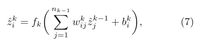
where 1≤k ≤K,i=1,2,...,nk.At the 1st layer:

wherei=1,2,...,n1.At the last layer:

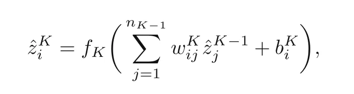
wherei=1,2,...,nK.wijandbidenote the weights and biases,respectively.jrefers to the position of node in the layer,andnk−1is the number of nodes at the (k −1)th layer.Thus,the output could be written in a tensor form:

2.2.2 Deep Lagrange method

The idea of how to find the minimum of the objective function under constraint conditions is given in Algorithm S3 (electronic supplementary materials).A deep neural network-based method finds the minimum of variables by solving Lagrangian duality function.The constraint conditions ˆgj ≤0 need to be checked before obtaining the output of the neural network.Then,the loss function,which is the output of the neural network at each iteration(or epoche),is defined as

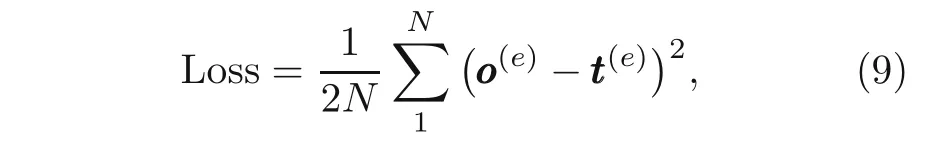
or it could be written as

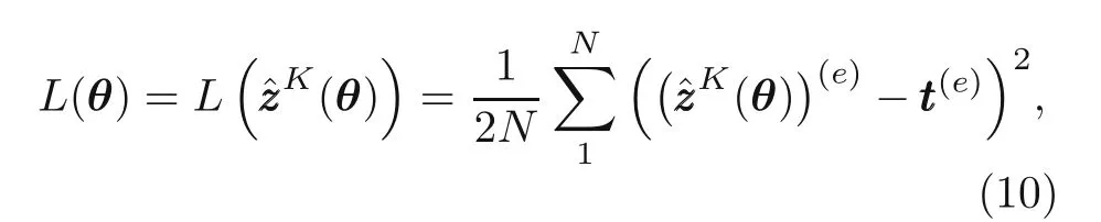
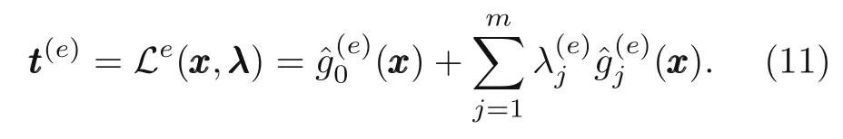
whereθdenotes the parameter set(weight and bias)of the neural network,Nis the number of neurons at the output layer,andtttis the target.The target and the Lagrange duality function at neural network iteration,e,are given as

In a deep neural network,the optimization problem is non-convex (Jain and Kar,2017).Gradientbased methods are used for convex problems in most cases as mentioned earlier(Boyd and Vandenberghe,2004).In this study,the Adam optimization algorithm(Kingma and Ba,2014)was used,which is one of the gradient-based methods,and was found to effi-ciently find local minima with high accuracy.We also tested the mini-batch (the default 32 mini-batch)(Bengio,2012).All the input data were normalized in the min-max normalization technique.The sigmoid activation function was employed for all layers,and the bias was set to zero,b1=b2=...=bK=0.

3 Numerical application to structural optimization

3.1 Weight minimization of a truss

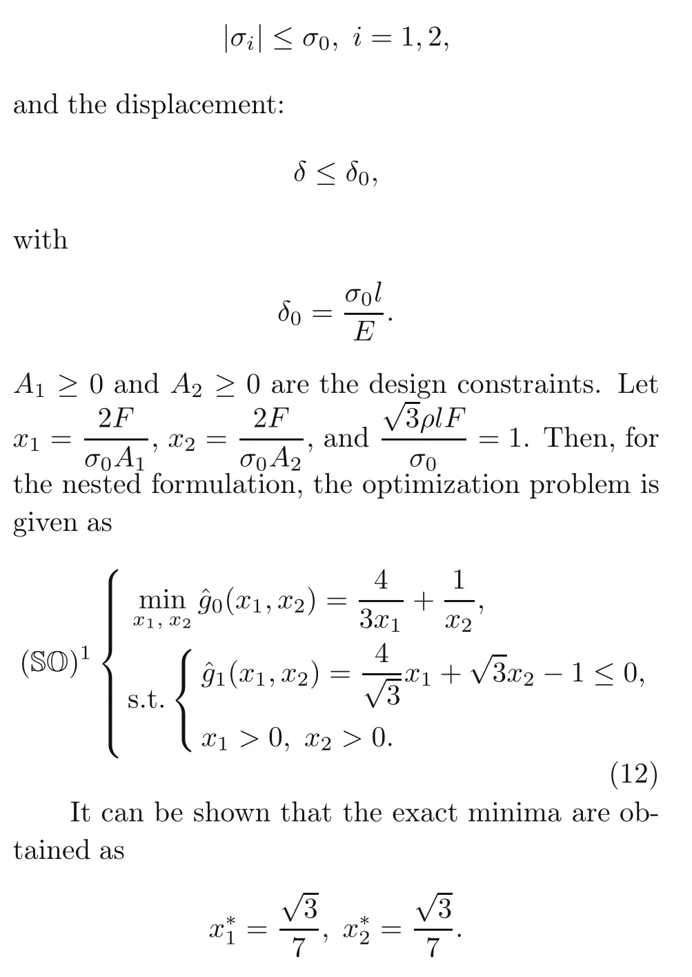
Let us consider the truss structure with Young’s modulusEand densityρ.Two bars of the truss connect at one end and join at an angle ofαas shown in Fig.3,wherelis the length of the first bar.A forceF >0 is applied to the truss.The objective of the problem was finding the cross-section areaAiof the two bars such that the weight is optimized.Furthermore,we impose constraint conditions on the maximum stress and displacement at the tipδ(Christensen and Klarbring,2009).

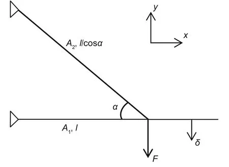
Fig.3 A truss of two bars subjected to stress constraints and tip displacement constraints

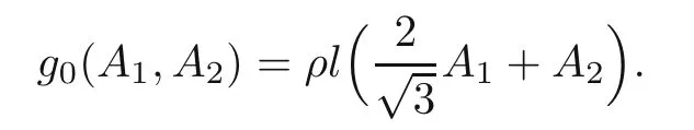
The weight of the truss is given by

Moreover,we require the following constraints on the stress:

The MMA,SLP with trust region strategy,and MPEA (Canfield,2018) are applied to solve numerically the test case.The derivatives of the objective functionand constraint functionwith respect toxiare needed to obtain the numerical results through these methods.The derivativeis computed as

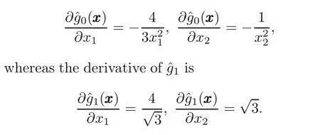
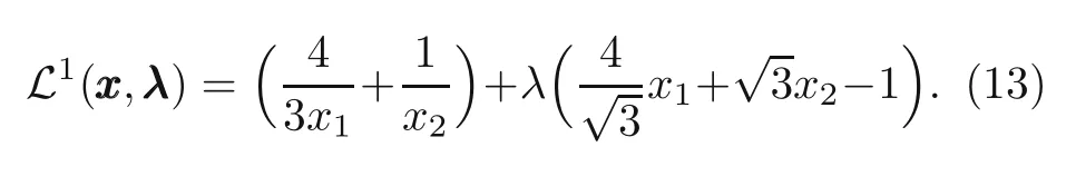
The numerical results of the MMA,SLP,and MPEA methods are summarized in Table 1.We first need to re-formulate the nested formulation in the Lagrangian duality form to solve this problem with the DLM,which can be written as

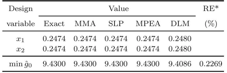
Table 1 Solution from the methods

To initialize the hyper-parameters,we follow the idea by Kingma and Ba (2014).Five hidden layers are used in which each layer has 10 hidden nodes.One thousand epochs are needed to iterate the network.We limit the range ofxi,that is,0.01≤x1,x2≤3 because the predicted result is in this range.A huge number of input data will be created if the large range ofxiis made (e.g.0.01≤xi ≤10).It,therefore,costs memory.The accuracy of the method depends on the interval size of the input,Δxi(Fig.4a),not the input range size ofxi.The choice of a large range size guaranteesto find the result.Also,we limit the range ofλas 0≤λ ≤15(Figs.4c and 4d).

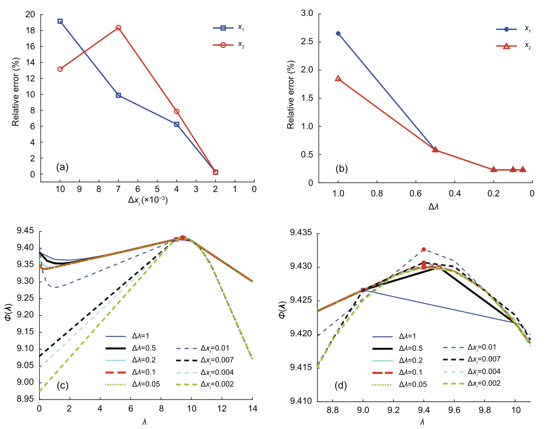
Fig.4 Relative errors of the solutions in terms of reducing the value of interval Δxi (a) and the value of interval Δλ (b),and the effect of choosing Δxi and Δλ in finding φmax (c) and the close-up peak of φ(λ) (d)

A technique of reducing the range of inputxiis used to reduce the number of input data sets as shown in Algorithm S1 (electronic supplementary materials).The first run following Algorithm S3 with the range 0.01≤x1,x2≤3,and Δxipredicts the optimum.Then the range of inputxiwill be reduced if the absolute error between the optimum value and that in exact solution (or numerical solution) is greater than a small positive tolerance∊;51 376 training sets are employed,and the global minimum of the solution is reported in Table 1.

The ranges of input data andλcould have been split into smaller ranges,that is,into the intervals Δxiand Δλ,instead of varying the number of input dataxiandλ(Fig.5).The smaller the intervals Δxiand Δλare,the larger is the number of input data to neural network.The solution when the range ofxihas different intervals is shown in Fig.4a.The accuracy of the result improves with decreasing interval Δxi(at Δλ=0.2).The smallest relative error of 0.2269% (Table 1,Fig.4a) is obtained for an interval value of Δxi=0.002.It is similar when obtaining the accuracy of the results with reducing interval Δλ(where Δxiis set to 0.002,Fig.4b).The interval value of Δλ=0.2 is small enough to obtain the accurate peak ofφ(λ).Figs.4c and 4d show how to find the maximum ofφ(λ)from the intervals Δxiand Δλ.It reaches the closest exact approximation point at the smallest interval of Δxiand small enough interval of Δλ(among the given intervals).

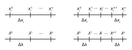
Fig.5 Variation of the intervals of the inputs, xi andλ

3.2 Weight minimization of a cantilever

Next,we consider a cantilever beam as depicted in Fig.6.The thin-walled cross-section can be found in Fig.6b,where the thickness is indicated bytand the length of the side of cross-section for each segment isxi,i=1,2.The aim of the problem was to findxiof the bars such that the weight is optimized under the constraint that the tip displacementδremains below a specified valueδ0(Christensen and Klarbring,2009).

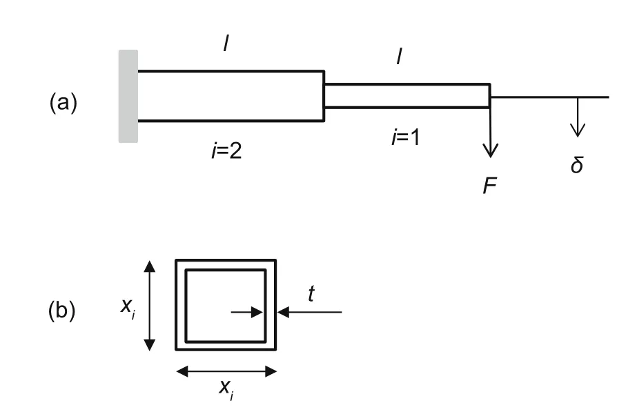
Fig.6 Two-bar cantilever beam (a)and hollow square cross-section of the ith segment (b)

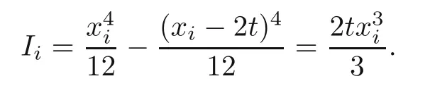
It is assumed that the thickness of the segment is small compared with the side length of the segment,t ≪xi.Thus,the second moment of inertia is calculated as

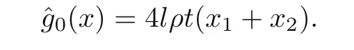
Then the weight of the beam is given by

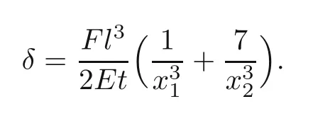
The tip displacement can be easily obtained by(Christensen and Klarbring,2009)

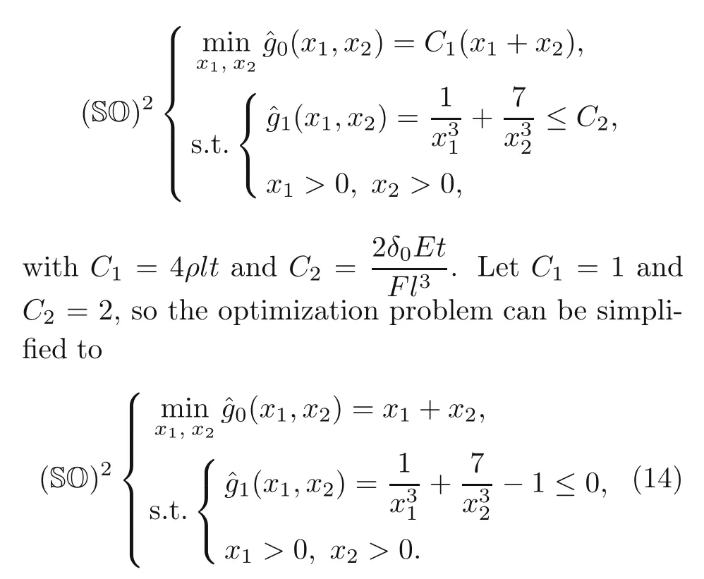
The optimization problem for the nested formulation is given by

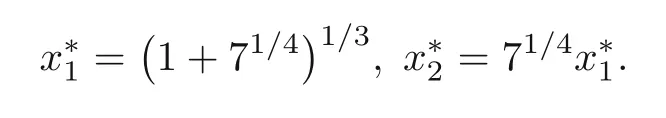
It is easy to show that the exact minimum values are

In Table 2,the results of the MMA,SLP,and MPEA methods can be found.

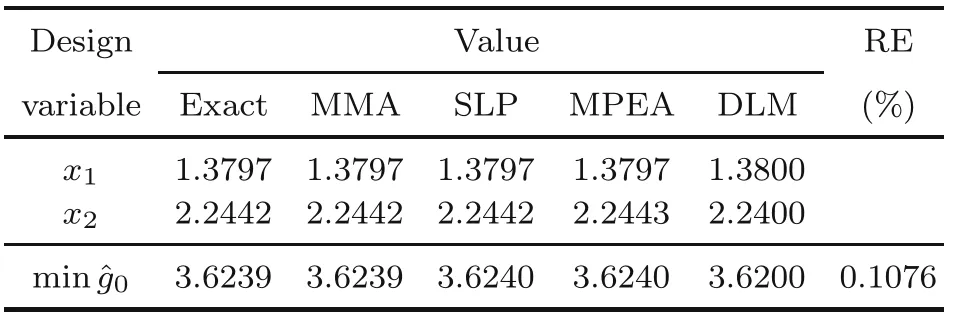
Table 2 Solution from the methods

We again first re-formulate the nested formulation into the Lagrangian duality form for the DLM method,given by

We again set ranges forxi,that is,0.1≤x1,x2≤5 and 0≤λ ≤5,which guarantees the global minimum;Δxi=0.02 and Δλ=0.1 are considered for input data to neural network.Five hidden layers,10 hidden nodes at each layer,and 1000 epochs are employed as in the previous example;103 275 training sets are applied into the input of the neural network after the range-reduction technique.In Table 2,the DLM solution is given,showing good agreement with the exact solution.

3.3 Sizing stiffness optimization

The truss shown in Fig.7 is considered next.Our aim was to maximize the stiffness of the truss,which is identical to minimize its complianceCCC=FFFTuuu,whereFFFis the external force vector anduuuthe displacement vector of the nodes of the truss.

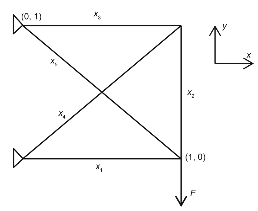
Fig.7 Five-bar truss under the sizing stiffness optimization

The nested optimization problem is finally written as

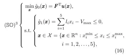
with an implicit functionxxx →uuu(xxx),which is defined from the equilibrium equationsKKK(xxx)uuu(xxx)=FFF.The bariof the truss has its lengthliand its crosssectional areaxi;Vmaxis the prescribed maximum volume of the truss structure.In this study,KKK(xxx)is the global stiffness matrix of the truss,and we assume that the global forceFFFdepends only on the design variablexxx,which is the cross-sectional area of the bars.

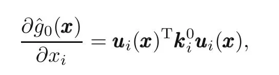
whereuuuiis the displacement of theith bar andis theith bar stiffness matrix (Christensen and Klarbring,2009),and the derivative of the constraint function is given as

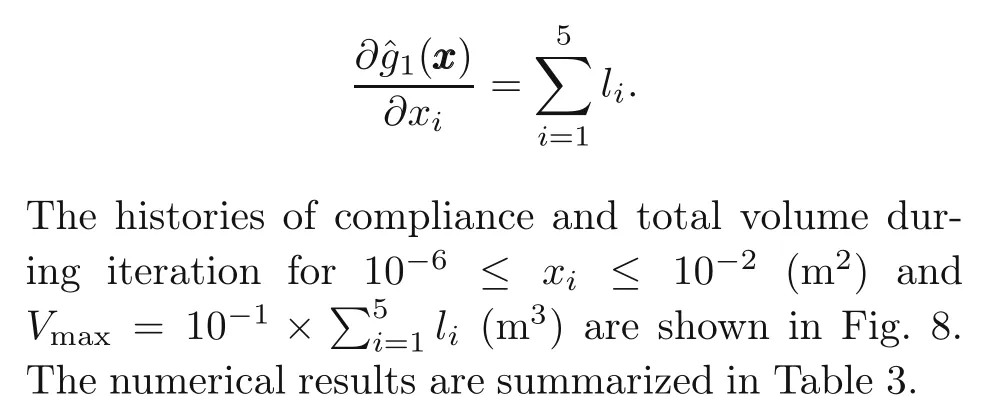
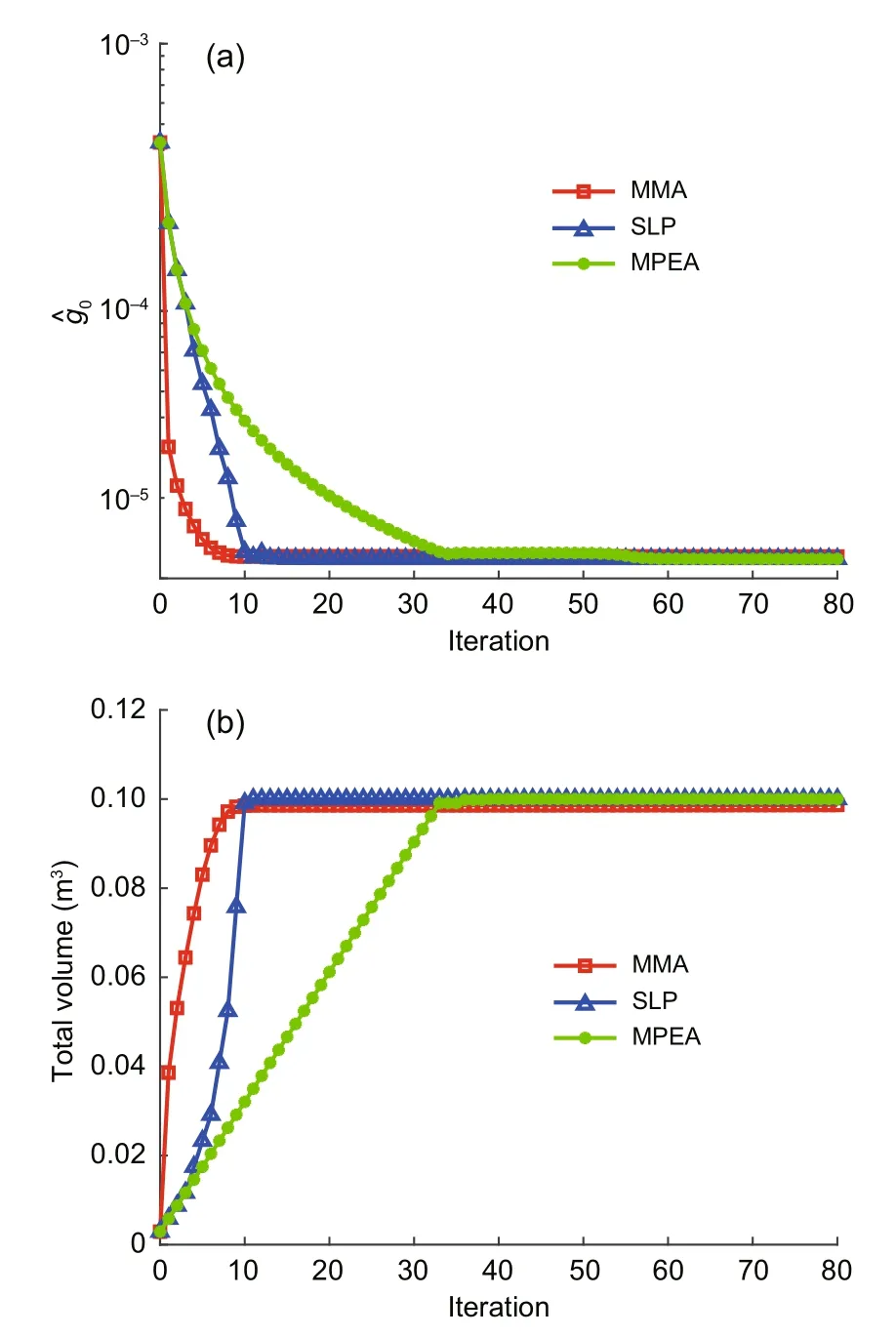
Fig.8 Histories of compliance (log scale on y-axis)(a) and total volume (b) after iterations

The Lagrangian duality form based on the optimized nested formulation is written as

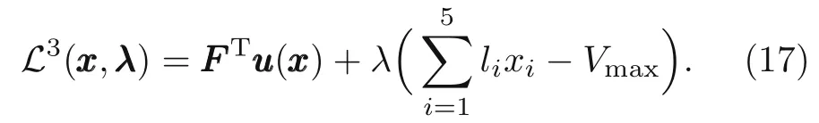
The range ofxiis chosen as 10−6≤ xi ≤10−2(m2) and the range ofλis 0≤λ ≤2 in the DLM initialization.The number of input data in training is obtained by setting Δxi=2×10−4and Δλ=0.1.Five hidden layers with 10 hidden nodes are employed,and 4000 epochs are employed in the iteration;688 128 training sets are applied to the input of the neural network after the range-reduction technique.The result of the DLM approach is depicted in Table 3,which agrees well with the numerical solutions.

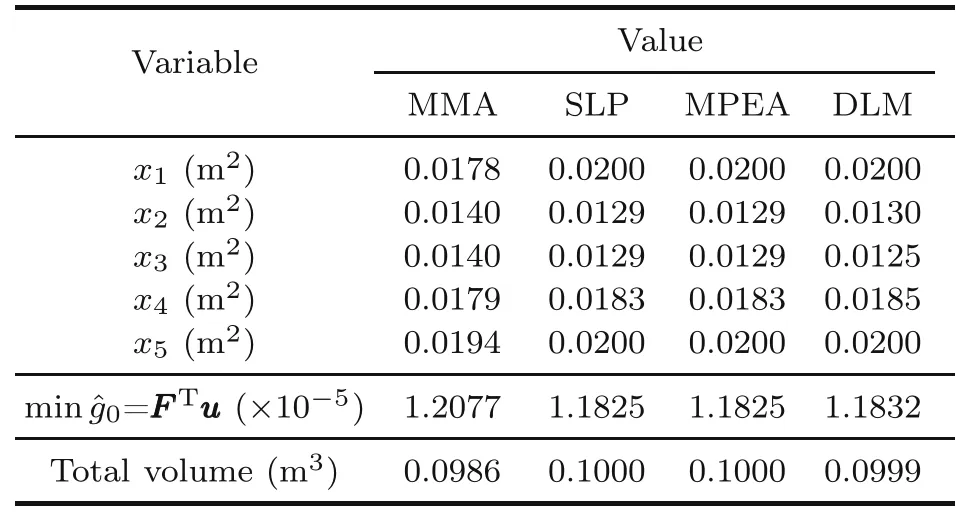
Table 3 Solution from the methods

3.4 Shape stiffness optimization

Finally,let us focus on a shape optimization problem of a sheet.It has the dimensions ofl,h,andt,as illustrated in Fig.9a.The left-hand side of the sheet is fixed,and the upper-side subjected to a distributed force ¯p.Again,we consider a linear elastic isotropic solid with Young’s modulusE,densityρ,and Poisson’s ratioν.The aim was to maximize the sheet’s stiffness,that is,to minimize the compliance.A constraint is imposed on the weight of the sheetWsheet,which is not permitted to exceed a prescribed value ofWmax.

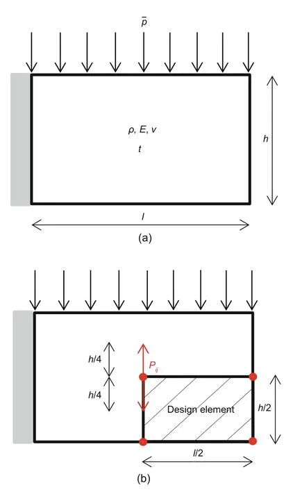
Fig.9 Sheet optimization problem (a) and the region of the sheet to be controlled (b)

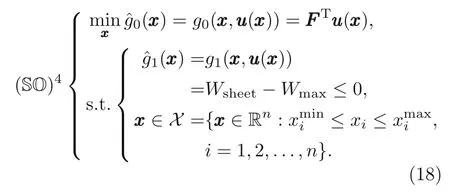
The nested optimization problem similar to the previous problem can be written as

We employ the finite element method to discretize the domain.The sensitivities are required in MMA,SLP,and MPEA.The nodal sensitivities are obtained through the partial derivatives at the nodal positions over the design variables.The boundaries become jagged (Christensen and Klarbring,2009)with the choice of using finite element nodes as design variables.Besides,it is an expensive computation when the mesh is fine.This fine mesh generates a large number of design variables (which are finite element nodes).Braibant and Fleury (1984) introduced B-spline curve technique in shape optimization to overcome this disadvantage.A very smaller number of design variables are carried out (control points in Fig.10) when using this curve technique.In practices,good results are archived using loworder B-spline polynomial function(Christensen and Klarbring,2009).Note that we employ second-order B-spline functions to discretize the boundary of the domain.

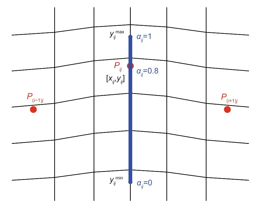
Fig.10 Control points including their spans

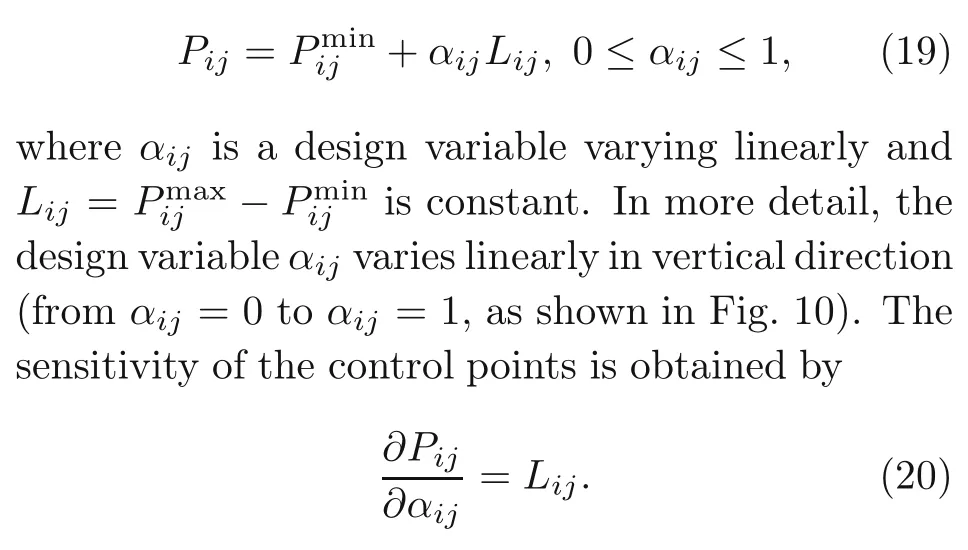
Let us consider the control pointPij=[xij,yij],i=1,2,...,nP,j=1,2,...,mP.Its location is given at

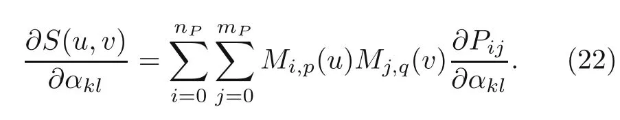
A B-spline surface is defined as(Piegl and Tiller,1997;Rogers,2001)

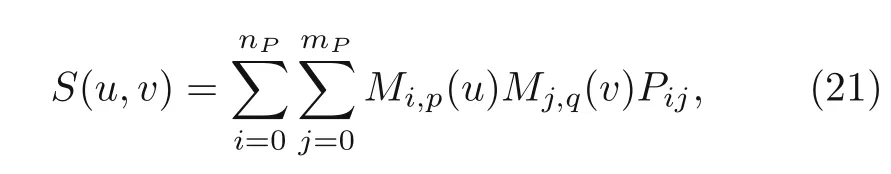
with basis functionMi,p(u) of polynomial degreepandr+1 number of knots;Mj,qis of polynomial degreeqands+1 number of knots.Therefore,the number of design variables are reduced to the number ofαijinstead of the whole number of finite element nodes.The derivatives of the B-spline surface over design variablesαklare given as

We employ numerical optimization methods and the DLM to solve the nested shape optimization problem (Eq.(18)).The associated algorithms are summarized in Algorithms S2 and S4(electronic supplementary materials).

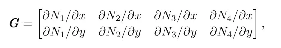
Note thatBBBdenotes the strain displacement matrix,DDDis the stress strain matrix,NNNis the matrix containing the shape functions (NNN=[N1N2N3N4]T) whileJJJindicates the Jacobian matrix in Algorithm S4.The area in the physical domain isΩ,whereasXXX′contains the nodal coordinates of elemente,and the derivative matrix of the shape functions is

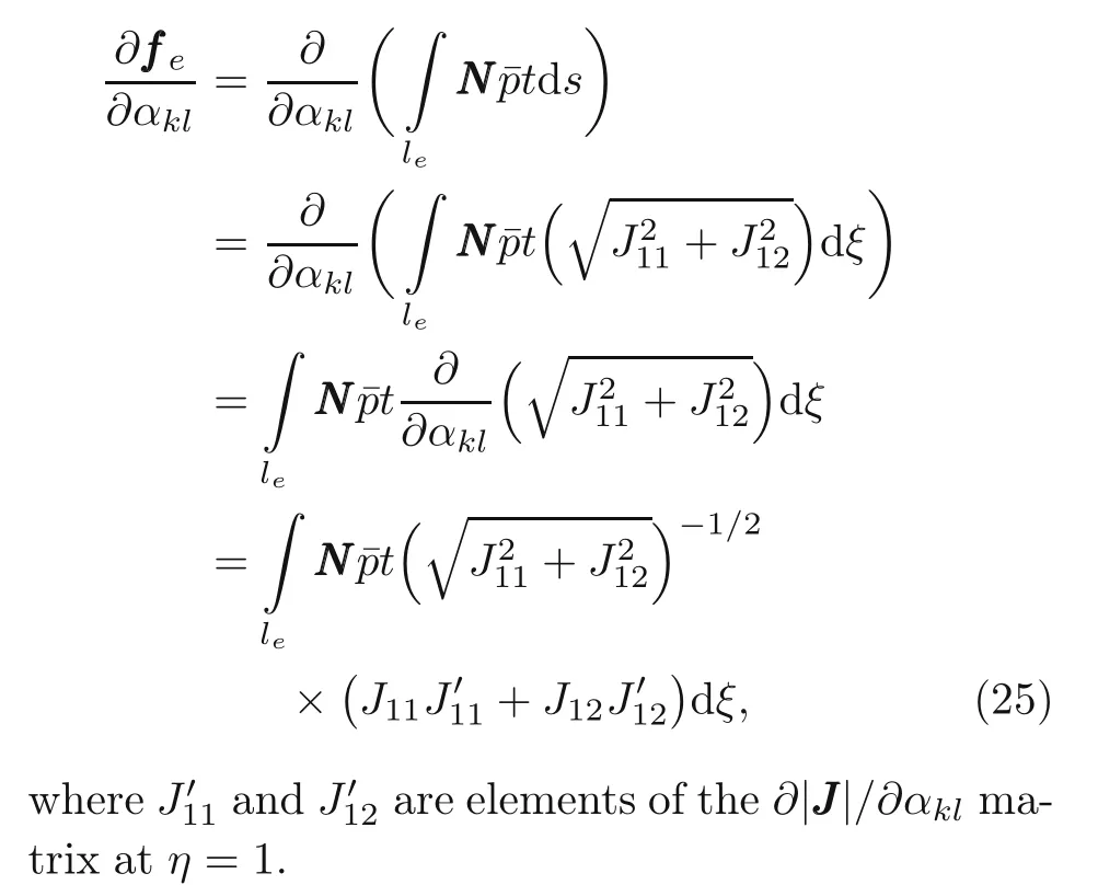
with∂BBB/∂αkland∂GGG/∂αkl(Haslinger and Mäkinen,2003).The forcefffeis expressed as

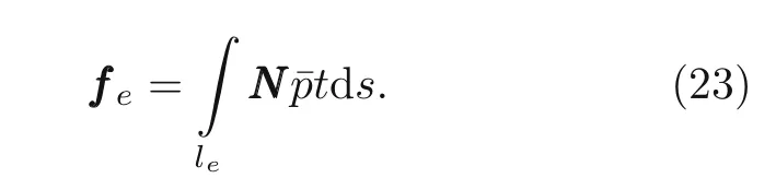
The differential of length on the top side,η=1,is expressed as

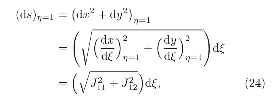
whereξandηare the isoparametric coordinates,andJ11andJ12are elements of the Jacobian matrix atη=1.Hence,the sensitivity analysis of the surface force can be expressed as

To test the problem,let us consider the four active control pointsPijshown in Fig.9b.They can move vertically up and down in the limit range[−h/4,h/4].Let the dimension of the sheet be asl=27,h=15,andt=1,and its material properties beρ=1,E=108,ν=0.3,and the maximum weightWmax=380.The histories of the compliance function and the weight versus iteration for the MMA,SLP,and MPEA methods are shown in Fig.11.Fig.12 shows the shape of the sheet after 60 iterations through MMA.

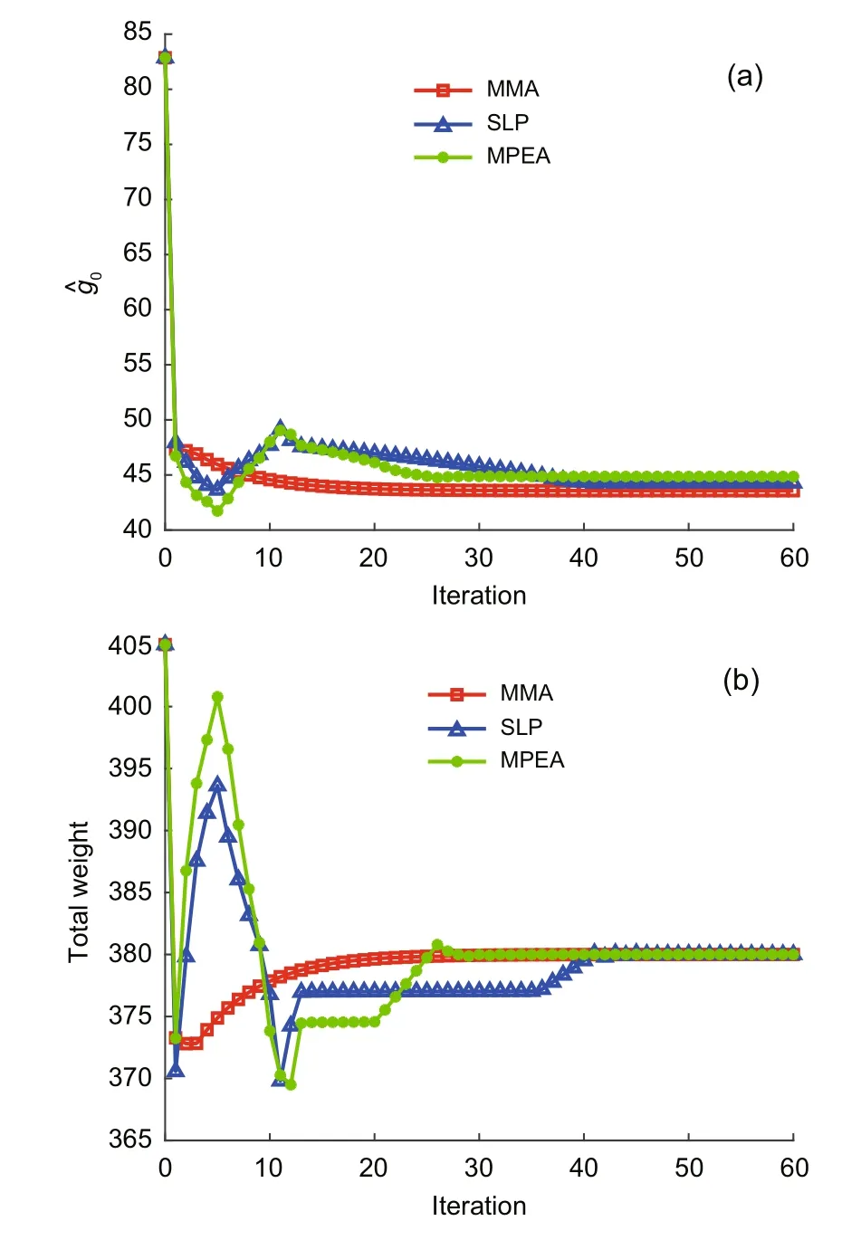
Fig.11 Histories of compliance (a) and total weight(b) after iterations

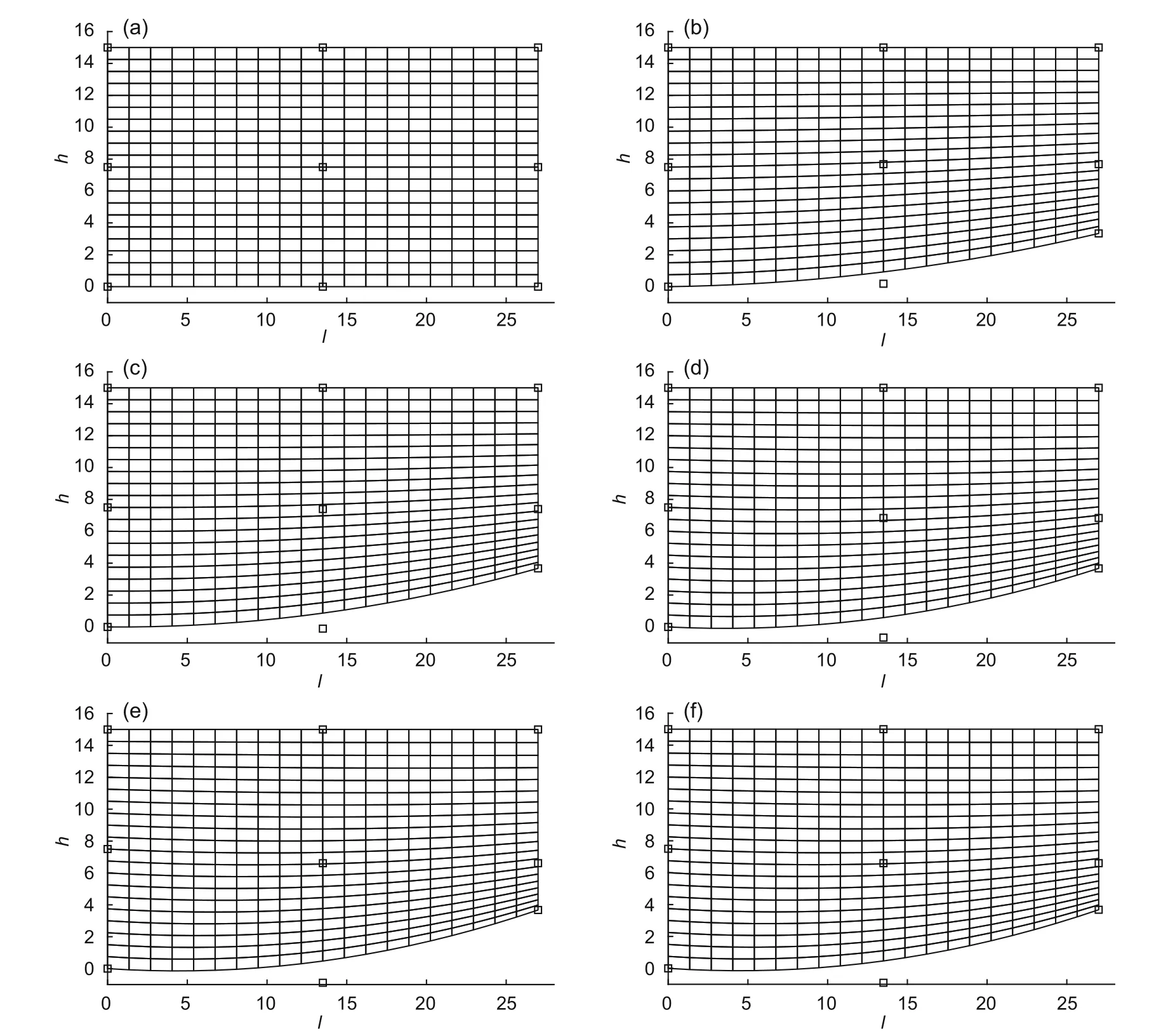
Fig.12 Shapes of the sheet after different numbers of iterations through MMA:(a) 0;(b) 1;(c) 3;(d) 10;(e)25;(f) 60

For the DLM,we employ five hidden layers,10 hidden nodes per layer,and 269 001 training data sets;3000 epochs are employed in the iteration.Also,the hyper-parameters are initialized follows the suggested configuration in(Kingma and Ba,2014).Table 4 shows the results for the DLM method compared with those of the MMA,SLP,and MPEA methods.The results are quite similar.

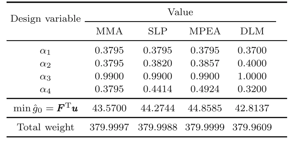
Table 4 Solution from the methods

4 Conclusions

We present a DLM for optimization problems in this study.They are based on minimizing the deep Lagrange functions.To demonstrate the capability of the method,we provided several examples of sizing and solved shape optimization problems,which are compared with exact solutions and solutions of the MMA,SLP,and MPEA.

DLM method applies Lagrange duality,which is a method to solve the optimization problems.However,this method requires derivatives in solving the problem.In finding the optimum solution,the idea of the DLM method is taking advantage of the neural network.One advantage of the DLM for sizing and shape optimization problems is the fact that it does not need a sensitivity analysis,which can be sometimes difficult to perform.One disadvantage of the proposed method is the potentially huge number of input data for the neural network.The approach is also limited by the number of design variable inputs due to the increasing amount of input datasets making the method computationally expensive.

When the number of design variables is small,i ≤3,the amount of input data is not large;therefore,it does not affect finding the optimum of the solution (Tables 1 and 2).The results are similar to those in the MMA method and the other two numerical optimization methods when more design variables are added (Tables 3 and 4).The accuracy of the method depends on the interval size of the input.The smaller the interval input size,the larger the amount of the input dataset for the neural network is employed.Therefore,a more advanced technique for reducing the number of input datasets has been developed to be applied to solve the structural optimization problem that requires a large number of variables.In the future,we intend to extend the approach to topology optimization problems.

Contributors

Dung Nguyen KIEN designed the research,processed the corresponding data,and wrote the first draft of the manuscript.Xiaoying ZHUANG revised and edited the final version.

Conflict of interest

Dung Nguyen KIEN and Xiaoying ZHUANG declare that they have no conflict of interest.

Acknowledgments

The authors would like to express the appreciation to Prof.Dr.Krister SVANBERG (KTH Royal Institute of Technology,Sweden) for his MMA codes,and Prof.Dr.-Ing.Timon RABCZUK (Bauhaus-Universität Weimar,Germany)for his critical comments on the manuscript.