Martingale Transforms on Variable Exponents Martingale Hardy-Lorentz Spaces
2021-06-30 00:07ZHANGChuanzhou张传洲JIAOFan焦樊ZHANGXueying张学英
应用数学 2021年3期
ZHANG Chuanzhou(张传洲),JIAO Fan(焦樊),ZHANG Xueying(张学英)
(College of Science,Wuhan University of Science and Technology,Wuhan 430065,China)
Abstract:In this paper,we research martingale Hardy-Lorentz spaces with variable exponents.Using the technique of Burkholder’s martingale transforms,the interchanging relations between two martingale Hardy-Lorentz spaces with variable exponents and BMO spaces with variable exponents are characterized,respectively.
Key words:Martingale transform;Hardy-Lorentz space;BMO space;Variable exponent
1.Introduction
The motivation in this paper comes from the classical results of CHAO and LONG[1-2],as well as the similar results of Weisz[3-4].The concept of martingale transforms was first introduced by Burkholder[5].It is shown that the martingale transforms are especially useful to study the relations between the predictable Hardy spaces of martingales,such as,which is associated with the conditional quadratic variation of martingales.
Lorentz spaces which were first introduced by Lorentz in 1951 have attracted more and more attention.Recently,the study of the martingale properties of Hardy-Lorentz spaces has become one of the hot topics and many important results have been obtained.FAN et al.[6]discussed Hardy-Lorentz spaces’basic properties,embedding relations and interpolation spaces.JIAO et al.[7]studied the atomic decompositions of Hardy-Lorentz spaces.In[8-9],the dual spaces of Hardy-Lorentz spaces are identified for real-valued and vector-valued martingales,respectively.HE[10]discussed the martingale transforms between Hardy-Lorentz spaces.
It’s well known that variable exponents Lebesgue spaces have been got more and more attention in modern analysis and functional space theory.Diening[11]and Cruz-Uribe[12]proved the boundedness of Hardy-Littlewood maximal operator on variable exponents Lebesgue function spacesLp(·)(Rn)under the conditions that the exponentp(·)satisfies so called log-Hlder continuity and decay restriction.
The situation of martingale spaces is different from function spaces.For example,the good-λinequality method used in classical martingale theory can not be used in variable exponent case.Aoyama[13]proved some inequalities under the condition that the exponentp(·)isF0-measurable.Nakai and Sadasue[14]pointed out that theF0-measurability is not necessary for the boundedness of Doob’s maximal operator,and proved that the boundedness holds when everyσ-algebra is generated by countable atoms.
The main purpose of this paper is to study martingale transforms on variable exponents martingale Hardy-Lorentz spaces.
2.Preliminaries and Notations
Letp(·):Ω→(0,∞)be anF-measurable function.We define

Moreover,whenp(·)≥1,we also define the conjugate functionp′(·)by=1.LetP(Ω)denote the collection of allF-measurable functionsp(·):Ω→(0,∞)such that 0<p-≤p+<∞.
The Lebesgue space with variable exponentp(·)denoted byLp(·)is defined as the set of allF-measurable functionsfsatisfying

where

For anyf∈Lp(·),we haveρ(f)≤1 if and only if‖f‖p(·)≤1.
We present some basic properties here:
1)‖f‖p(·)≥0,‖f‖p(·)=0⇔f≡0;
2)‖cf‖p(·)=|c|·‖f‖p(·)forc∈C;
3)For 0<b≤min{p-,1},we have
Letp(·)∈P(Ω)and 0<q≤∞.ThenLp(·),q(Ω)is the collection of all measurable functionsfsuch that

According to Theorem 3.1 in[15],the spacesLp(·),qare quasi-Banach spaces.Moreover,it is similar to the classical case that the equations above can be discretized:

and

Let(Ω,F,P)be a complete probability space,andFnbe a nondecreasing sequence of sub-σ-algebra ofFsuch thatwhereFnis generated by countably many atoms.The conditional expectation operators relative toFnare denoted byEn.
We point out that,our results heavily rely on the following condition:There exists an absolute constantKp(·)≥1 depending only onp(·)such that

whereA(Fn)denotes the family of all atoms inFnfor eachn∈N.
For a complex valued martingalef=(fn)n≥0relative to(Ω,F,P;(Fn)n≥0),denotedfi=fi-fi-1(with conventiondf-1=0,F-1={Ω,∅})and

Thus the variable exponents martingale Hardy-Lorentz spaceis defined by

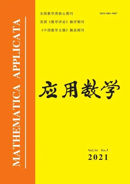
Definition 2.1Define the following classes of processesv=(vn)n≥-1adapted to(Fn)n≥-1by
whereM(v)=supn≥-1|vn|.The martingale transform operatorTvfor given martingalefandv∈Vp(·),qis defined byTv(f)=(Tv(fn))n≥0,where

Leth(λ)=‖χ{|f|>λ}‖p(·),f*(t)=inf{λ>0:h(λ)≤t},dt.
Definition 2.2A bilinear operaorTis a convolution operaor if and only if forh=T(f,g),

As the proof of Theorem 2.6 in[16]we also have
Theorem 2.1For allf∈Lp2(·),q2,g∈Lp(·),q,0<p+0<q,q2≤∞,with

3.Boundedness of Martingale Transform Operators
In this section,we investigate the boundedness of martingale transform operators on spacesBMO2(α(·)),respectively.
Definition 3.1Letα(·)+1∈P(Ω)be a variable exponent and 1<q<∞.DefineBMOq(α(·))as the space of all functionsf∈Lqfor which

is finite.Forq=1,we defineBMO1(α(·))with the norm

Definition 3.2Let 1≤r<∞,0<q≤∞andα(·)+1∈P(Ω).The generalized martingale spaceBMO2,q(α(·))is defined by

where

and the supremum is taken over all atoms{Ik,j,i}k∈Z,j∈N,isuch thatIk,j,iare disjoint ifkis fixed,Ik,j,ibelongs toFjifk,jare fixed,and

The following lemmas can be seen in[17].
Lemma 3.1Letp(·)∈P(Ω)satisfy the condition(2.4),0<p+≤1 and 0<q≤1.Then

Lemma 3.2Letp(·)∈P(Ω)satisfy the condition(2.4),0<p+<2 and 1<q<∞.Then

Theorem 3.1 Letp(·),p2(·)∈P(Ω)satisfy the condition(2.4),0<q,q2<∞,v∈Vp(·),qwithandThenTvis of typewith‖Tv‖≤c‖v‖Vp(·),q.
ProofUsing the pointwise estimation


This means thatTvis of typewith‖Tv‖≤c‖M(v)‖p(·),q=c‖v‖Vp(·),q.
Theorem 3.2Letp(·)∈P(Ω)satisfy the condition(2.4),1<q<∞,α(·)<andv∈Vp(·),q.ThenTvis of type(BMO2(α(·)),whereβ(·)=.
ProofSetp1(·)==1.We can choose 1<p2(·)<2 such thatIt is well known thatTvis a self-adjoint operator on Hilbert spaceL2and E(fTv(φ))=E(φTv(f))for anyφandfinL2(see[2]).Since 1<p2(·)<2 andL2is dense in(see Remark 3.8 in[17]),we have

Consequently,for anyφ∈BMO2(α(·)),f∈(1<p2(·)<2),by Lemma 3.1 and Theorem 3.1 we can see


This means thatTvis of type(BMO2(α(·)),with‖Tv‖≤c‖v‖Vp(·),q.
4.Relations Between and
Suppose thatA0andA1are quasi-normed spaces,embedded continuously into a topological vector space.The interpolation spaces betweenA0andA1are defined by means of the socalledK-functionalK(t,f;A0,A1).Iff∈A0+A1,setK(t,f;A0,A1)=inff=f0+f1{‖f0‖A0+t‖f1‖A1}.The infimum is taken over all possible decompositions withf=f0+f1,fi∈Ai,i=0,1.The interpolation space(A0,A1)θ,qis defined as the space of all functionsf∈A0+A1such that

Lemma 4.1[17]Letp(·)∈P(Ω),0<q≤∞,0<θ<1 andThen

Then,for anyf∈we have the following decomposition

Theorem 4.1Letp1(·),p2(·)∈P(Ω),0<p1(·)<p2(·)<∞and 0<q<∞.Suppose thatone of its martingale transformg=Tv-1(f)={gn}n≥0withwhere:=min{E(sj+1(f0)-β|Fj),1}for anyj≥-1,f0is given by(4.2)andThenand.
ProofFrom the definition ofit is easy to see that the proces sv-1=is adapted to{Fj}j≥1and1 for everyj≥1.Theng={gn}n≥0is a martingale transform off={fn}n≥0with the multiplier sequencev-1=1.
Moreover,from(4.2)and the decomposition off,the martingaleghas the corresponding decompositiong=g0+g1,such that


Then

This proves that


Consequently,we have

Thus we have

So

Then

Thus we complete the proof of Theorem 4.1.
Similarly,we have the following theorem and we omit the proof of it.
Theorem 4.2Letp1(·),p2(·)∈P(Ω),0<p1(·)<p2(·)<∞and 0<q1<q2<∞.Suppose thatone of its martingale transformg=Tv-1(f)={gn}n≥0with

5.Relations Between and BMO2
Theorem 5.1Let 1<p(·)≤2,0<q<∞.Then for anythere exist a martingaleg∈BMO2with‖g‖BMO2≤1 andv∈Vp(·),qwithsuch thatf=Tv(g).Conversely,for anyv∈Vp(·),qandg∈BMO2,the martingalef=Tvgis inand.
ProofThe converse assertion follows from Theorem 3.2 immediately.For everyj≥-1,takevj=supm≤jE(s(f)|Fm)and define

Then,it is clear thatf=Tvgand{E(s(f)|Fn)}n≥0is a martingale.Denoting its maximal function byM(s(f))=supn<∞E(s(f)|Fn),we have

Applying Doob’s inequality for variable exponent martingale spaces and interpolation theorem,we have

This impliesv∈Vp(·),q.By Jensen’s inequality,we get

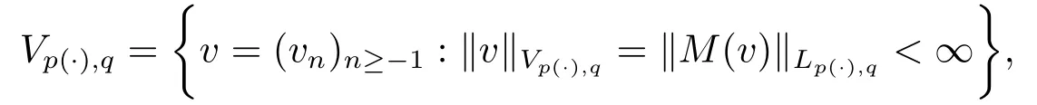
Hence,forN>n≥0,we have
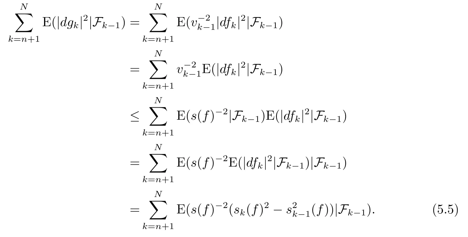
Therefore
Hence,we obtain thatg∈BMO2and‖g‖BMO2≤1.