Adaptive Maxwell’s Equations Derived Optimization and Its Application in Antenna Array Synthesis

Donglin Su,Lilin Li,Shunchuan Yang,Fei Wang

1 School of Electronics and Information Engineering,Beihang University,Beijing 100191,China

2 Research Institute for Frontier Science,Beihang University,Beijing 100191,China

3 Shenyuan Honors College,Beihang University,Beijing 100191,China

Abstract:In this paper,a self-adaptive method for the Maxwell’s Equations Derived Optimization(MEDO)is proposed.It is implemented by applying the Sequential Model-Based Optimization(SMBO)algorithm to the iterations of the MEDO,and achieves the automatic adjustment of the parameters.The proposed method is named as adaptive Maxwell’s equations derived optimization(AMEDO).In order to evaluate the performance of AMEDO,eight benchmarks are used and the results are compared with the original MEDO method.The results show that AMEDO can greatly reduce the workload of manual adjustment of parameters,and at the same time can keep the accuracy and stability.Moreover,the convergence of the optimization can be accelerated due to the dynamical adjustment of the parameters.In the end,the proposed AMEDO is applied to the side lobe level suppression and array failure correction of a linear antenna array,and shows great potential in antenna array synthesis.

Keywords:electromagnetic compatibility;Maxwell’s equations derived optimization;adaptive Maxwell’s equations derived optimization;sequential modelbased optimization;antenna array synthesis

I.INTRODUCTION

Optimization algorithms are utilized more and more broadly in recent years including the optimization algorithms based on gradient descent,the optimization algorithms inspired by natural phenomena,and the optimization algorithms derived from physical rules.In electromagnetics and communications,the optimization problems are usually high-dimensional,multimodal and complex,which are challenging for the optimization algorithms.In order to solve the optimization problems in the electromagnetics and communications more efficiently,Maxwell’s Equations Derived Optimization(MEDO)is proposed,which is one of the typical representatives of the third type of the algorithms[1].

Compared with other popular optimization algorithms such as Gradient Descent(GD)[2],Particle Swarm Optimization(PSO)[3,4],Differential Evolution(DE)[5],and Adaptive Wind Driven Optimization(AWDO)[6],MEDO can attain more accurate and more stable optimization results for both unimodal functions and multimodal functions[1].However,the performance of MEDO is sensitive to the parameters,which need to be tuned manually for different problems.Tuning the parameters manually is a timeconsuming and labor-intensive task because the optimization algorithm is considered as a black box solver for users.Once the parameters’values are set improperly,the performance of MEDO may be degenerated.To alleviate the issue,in this paper,we propose a selfadaptive method for MEDO to select the values of the parameters automatically,which is named as adaptive Maxwell’s equations derived optimization(AMEDO).

The rest of the paper is organized as follows.Section II briefly summarizes the MEDO.The Sequential Model-Based Optimization(SMBO)method which is used to adaptively adjust the parameters in the MEDO is outlined in Section III.Section IV presents the AMEDO algorithm.The numerical tests and results are shown in Section V and Section VI gives two examples of AMEDO when it is applied in the antenna array synthesis.The conclusion and the future works are stated in Section VII.

II.MAXWELL’S EQUATIONS DERIVED OPTIMIZATION

MEDO is an optimization algorithm,which evolves from the Law of Conservation of Charge and Faraday’s Law,and shows strong potential in the applications of electromagnetics[1].The algorithm is inspired by summarizing the behavior of the charged conductors in time-varying electromagnetic fields.It considers a long coaxial which is excited by a variable frequency source and ended with a matched load.A conductor with small resistance is used to connect the extremity and the source.If we inject signals of different frequencies on the coaxial,it can be observed that when the frequency is relatively low,the current flows back to the source through the conductor.When the frequency is high,the current chooses the outer sheath of the coaxial.

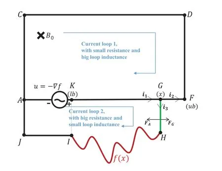
Figure 1.Schematic of MEDO.

The coaxial can be simplified to be a paralleled circuit.Its two branches represent the conductor loop and the coaxial sheath loop.Denote the two branches as loop 1 and loop 2,respectively.To adapt to the construction of the optimization algorithm,MEDO treats one segment in the loop 2 as an individual in the optimization to find the optimal solution,and treats the conductor connected to it as the region to be optimized.The simplified model is shown in Fifure 1,with the individual denoted as GH,and the optimized region marked as HI.The circuit is placed in a constant magnetic fieldB0.Assume that the value of the voltage source is equal to the negative gradient of the objective function,the current on GH can be calculated through the Law of Conservation of Charge and Faraday’s Law as shown as:

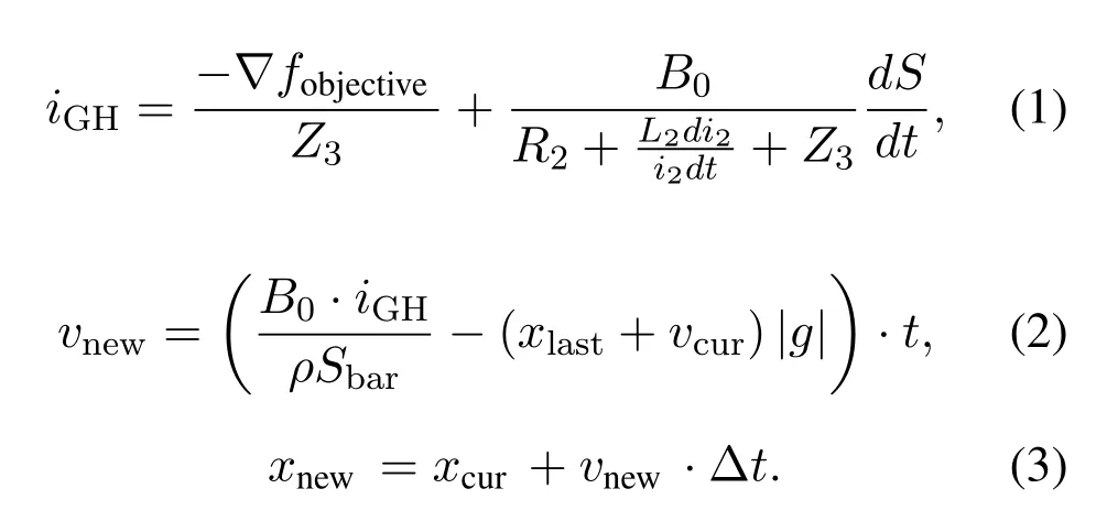
According to the Fleming’s Left rule,if the position of GH is allowed to be variable,it will move along the Ampere force.The velocity and the position update formula in MEDO can be derived from the momentum theorem,as shown in(2)and(3).

In(1)-(3),some parameters are needed to be known to obtainxnew.Among these parameters,some are calculated from the model,such asZ3,while the others are preset by the users.The parameters required to be pre-designed include|g|,B0,ρSbar,R1,andL2.They refer to the gravitational acceleration,the magnetic flux density,the per-unit-lengthweight of the conductor,the resistant of the main branch,and the loop inductance of current loop 1,respectively.Reference has proved that the individuals can converge to the optimal location of the objective function under the appropriate parameter settings[1].

III.SEQUENTIAL MODEL-BASED OPTIMIZATION

Sequential Model-Based Optimization is a kind of model-based optimization method,which builds a regression model to fit the objective function and predicts more detailed information about the objective function based on the model[7,8].SMBO does not need additional parameters and gradient information of the objective function,which makes it a good choice to adaptively adjust the parameters in the optimization algorithms.

In SMBO,additional data are gathered step by step in the iteration,which helps the predicted model to approach the actual objective function gradually.The procedure of SMBO can be understood by the following explanation of the two adjacent steps.In step one,assuming that some data have been sampled,SMBO finds a response surface model to fit the existing data,and searches for a value that maximizes the acquisition function.The searched value is added to the sampled points in step two.SMBO then calculates the objective function value of the searched point and updates the response surface model based on it.

The most common choice of the response model is Gaussian Process(GP)model[9,10],which assumes that the sampled data satisfy the Gaussian process.Given some certain sampled data,the possible probability distribution of the observed points can be calculated according to GP.The expected value and the uncertainty of the predicted model can be described by the mean and covariance matrices of the Gauss distribution.Base on the predicted GP model,the data with the maximum value of acquisition function can be selected as the next sampled data.As for the acquisition function,the usual choices include the probability of improvement(PI)[11],the expected improvement(EI)[12,13],and the upper confidence bound(UCB)[14].PI focuses on the probability that whether the objective function value of the sampled data is better than the optimal value known so far.However,it usually requires amounts of calculations in low explored areas to achieve the probability of improvement,making this acquisition function a little inefficient.EI is an expected function.It considers how much better the objective function value of the sampled data is than the current optimal solution,and chooses the data whose objective function value can most improve the solution as the next sampled data.This acquisition function is frequently used when the value of the objective function is noiseless.UCB acquisition function is a strategy of confidence boundaries,and balances the exploitation and exploration terms.In general,an adaptation of the hyper parameterκis needed to run the UCB normally.

IV.ADAPTIVE MAXWELL’S EQUATIONS DERIVED OPTIMIZATION(AMEDO)

4.1 Algorithm Descriptions

In MEDO,there are 5 parameters that need to be predefined before starting the optimization.The 5 parameters are named as|g|,B0,ρSbar,R1,andL2,respectively.The value of the parameters may affect the performance of MEDO.To illustrate this fact more intuitively,we have made some numerical tests as examples.One typical benchmark is calculated by MEDO,with each parameter varies independently.Other parameters take the best values suggested in[1].The

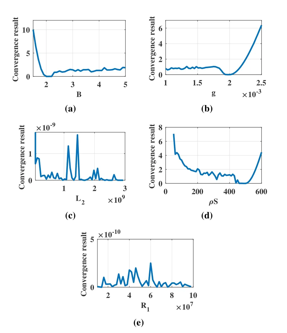
Figure 2.The curves of the convergence errors changing with the variation of each parameter.

curves of the convergence errors that change with the variation of each parameter are plotted in Fifure 2.It can be concluded that the performance of MEDO is sensitive to the independent change of each parameter.Presumably,the combination variations of the five parameters have a more serious impact.Certainly,when the objective function is changed,the corresponding optimal value range of each parameter is varied.Although in the related reference,some works have been done to understand the physical meaning of the parameters and their approximate range,it is a relatively difficult task to manually adjust them to obtain good performance in the MEDO in some unknown cases[1].

In this section,we propose a self-adaptive method to adjust the parameter values automatically,which can mitigate the issue of choosing the proper values for the 5 parameters manually.The SMBO method is applied here for this purpose.The response surface model of SMBO is supposed to be GP.By considering that the objective function is directly calculated without noise,we choose EI as the criterion of SMBO here.SMBO uses the same population size as MEDO,while the optimization problem space is only limited to five dimensions for the inherent parameters:|g|,B0,ρSbar,R1,andL2.In each iteration,SMBO returns new sets of the five parameter values for each member in the population according to the previous sampled points.

In addition,SMBO may suffer from overfitting due to the lack of sampled data or the excessive complexity of the model.In order to avoid overfitting of SMBO,we make two improvements in this work.

(1)A threshold is set to accumulate adequate sampled points before SMBO is applied to the parameter adaptation.The training samples are too few is one of the main reasons for overfitting.Therefore,when the iteration number is smaller than the threshold,the five parameters are updated randomly within the range suggested by the reference[1].SMBO is utilized to achieve the self-adaptation of the parameters when the iteration number is larger than the threshold.In order to determine the proper value of the threshold,we test the influence of the threshold value on the algorithm’s performance in section V,and choose the most suitable one.

(2)A feedback mechanism is set to terminate the poor updating of the parameters.After the adaptive parameters are applied in the MEDO,we compare the calculation result in the current iteration to the optimal solutions ever reached.If the optimal solution has not been updated for 10 consecutive times,the proposed method terminates the update of the parameters,and uses the optimal parameters known so far.

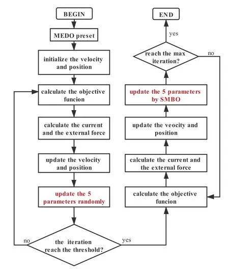
Figure 3.The flowchart of the proposed AMEDO.

The flowchart of the proposed AMEDO is illustrated in Fifure 3.It begins with the initialization of the algorithms,such as randomly generating position and velocity.Then,the objective function value of each individual in the population is evaluated.According to the objective function values,the external force on the slide bar is calculated.Then,the velocity along with the position is updated with the random parameters when the iteration number is smaller than the threshold.After the iteration number reaches the threshold,the objective function value of the population and the values of the five parameters are transferred to the SMBO algorithm,including the current values and the historical values.SMBO then selects a new set of values for the five parameters based on the predicted Gaussian model and the acquisition function.The iterative process of updating the population and parameters continues until the maximum number of iterations is reached.

4.2 Computational Complexity Analysis

The computational complexity of AMEDO mainly includes the calculations of the objective functions and their gradients,and the self-adaptation of the five parameters.DenoteP,Das the population size and the dimension of the objective function,respectively.The cost of the objective function calculations and the gradient calculations can be named as the MEDO part.According to the reference,the computational complexity of this part can be described asO(D×P)×O(f)in each iteration,whereO(f)refers to the calculation complexity of the objective function[1].In the parameter adaptation part,the computational complexity of the update for each parameter is proportional to the third order of its range.By considering that the ranges are different for different parameters,the maximal one of the five parameters’ranges is used to describe the computational complexity.In conclusion,the computational complexity of AMEDO can be approximately analyzed by combining the MEDO part and the parameters adaptation part together.

In most cases,the computational complexity of the objective function calculation is much larger than that of the parameter adaptation.Thus,we can mainly consider the computational consumption of the MEDO part in practice.

V.NUMERICAL TES TS

To evaluate the performance of the proposed AMEDO,8 benchmarks have been tested.The benchmarks include the unimodal functions and multimodal functions,which are frequently used to test the convergence capability of the optimization algorithms[15,16].The accuracy and stability of AMEDO are mainly investigated through multi independent tests of the benchmarks.Descriptions of the eight benchmarks are shown in the Table 1.

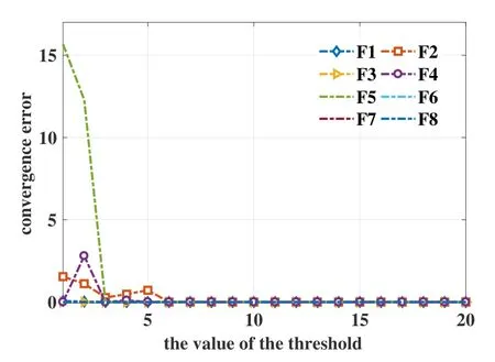
Figure 4.The effect of the threshold value on the accuracy.

Firstly,the influence of threshold value on the algorithm performance is tested,including the effect on the accuracy and the average iteration number needed for convergence.The results are shown in Fifure 4 and Fifure 5,respectively.They reveal that the value of the threshold almost has no obvious effect on the accuracy of the algorithm when it is larger than 6,while the number of iterations needed for convergence increases as the threshold increases.Thus,taking accuracy and convergence speed into consideration,the threshold is set to be 6 in the following tests.

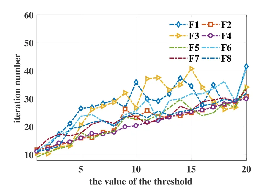
Figure 5.The effect of the threshold value on the iteration number needed for convergence.

Then,accuracy and stability of AMEDO are tested.Each benchmark has been run for 100 times,150 iterations every time starting from the random populations.The population size is set to be 60.In order to evaluate the change of the algorithm performance when the parameters are self-adaptive by SMBO,the origin MEDO has been tested in the same environment.The parameters of the original MEDO have been manually adjusted with a lot of efforts and time,which can make the MEDO maintain a satisfying performance.In general,we use the minimum error of the test results to represent the accuracy of the algorithm,and use the standard deviation of the errors of the results to represent the stability.The smaller minimum value means the higher accuracy,and the smaller standard deviation refers to the higher stability.The results are shown in Table 2.

From the results in Table 2,it can be concluded that AMEDO can converge to the results with the analogous accuracy and stability compared with the original MEDO.It is worth mentioning that AMEDO needs no external input of the parameters from the users,which can reduce the labor cost.

Additionally,in order to test and verify that whether the self-adaptation of the parameters can speed up the convergence of the optimization algorithm,the convergence processes of AMEDO and MEDO are drawn in the same figure.The blue line represents the convergence process of AMEDO,and the red one represents the convergence process of the original MEDO.

Table 1.The description of the benchmarks.

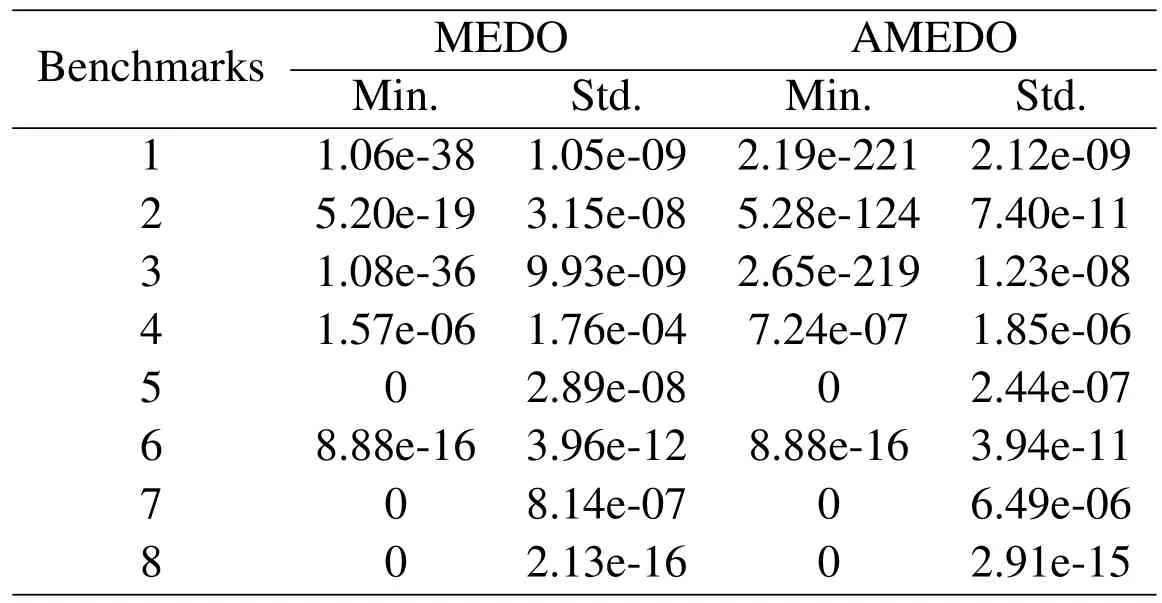
Table 2.Numerical test results of MEDO and AMEDO.

According to Fifure 6,AMEDO is proven to converge more rapidly than the original MEDO.When the calculation of the objective function takes a long time,the advantage of rapid convergence becomes particularly important.

VI.APPLICATIONS IN ANTENNA ARRAY SYNTHESIS

Antenna array synthesis is one of the most important tasks in communications.The proper design of the antenna array can obtain better antenna performance[17].For example,through the side lobe level(SLL)suppression,the antenna can obtain larger gain in the main lobe towards the expected signal[18-20].And the interference signals can be filtered out by placing the corresponding nulls toward the direction of interference signals.These design problems can be considered as optimization problems.The feature of this kind of problems is that there are many variables to be optimized,causing the search space multiplying and the error accumulating seriously.Thus,finding the optimal solutions of these optimization problems is difficult.

6.1 Side Lobe Level Suppression

AMEDO is used to suppress the SLL of a linear antenna array as the first example of its application in the antenna array synthesis.Assume that the linear array is placed along thex-axis symmetrically,which consists of 32 identical isotropic dipole antennas,then the array factor(AF)can be shown as:

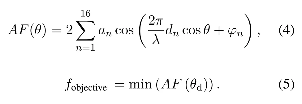
AMEDO is applied here to select the optimal amplitudes of the excitations and the element locations to achieve the SLL suppression.The objective function of this problem can be described as minimizing the side lobe level as demonstrated in(5).

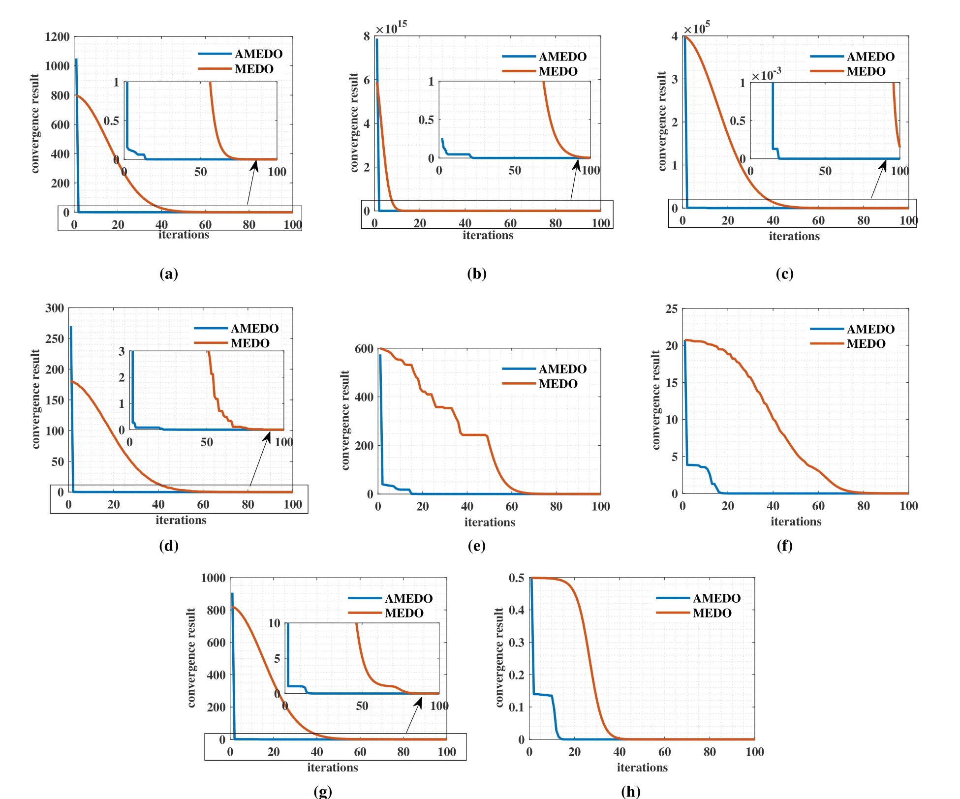
Figure 6.The convergence speed comparison of the proposed AMEDO and origin MEDO for the benchmarks:(a)F1;(b)F2;(c)F3;(d)F4;(e)F5;(f)F6;(g)F7;(h)F8.

In(5),θdis the angle where the SLL needs to be controlled.

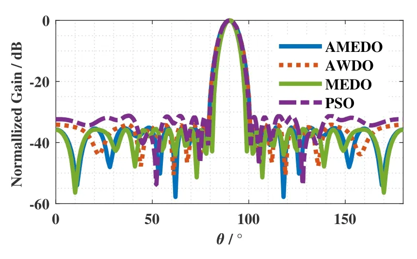
Figure 7.Normalized gain comparison between AMEDO,AWDO,MEDO and PSO.

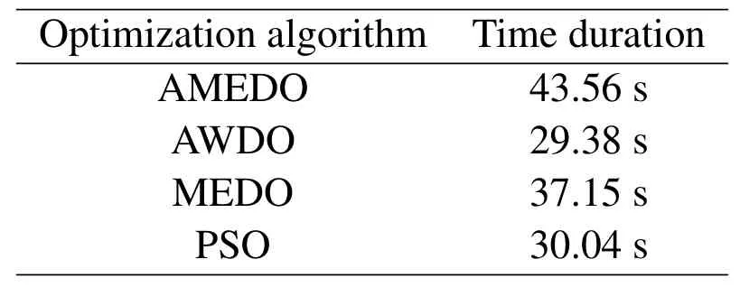
Table 3.Time duration of different optimization algorithms in SLL suppression.

Similar work has been done by the AWDO[6],the original MEDO[1]and PSO[20].The obtained results of the different optimization algorithms are shown in Fifure 7.From the results,it can be concluded that AMEDO can attain a more satisfying result(-35.55 dB)than AWDO(-34.16 dB)and PSO(-31.29 dB),and a matched result with the original MEDO(-35.71 dB),without tuning the parameters manually.

The calculation time durations of AMEDO,AWDO,MEDO and PSO are shown in Table 3 without considering the time spent on the parameters tuning manually.The condition of terminating the optimization algorithm is that the iteration number is larger than 100.

With this setup,the time durations of AMEDO and MEDO are longer than that of the optimization algorithms,because their time complexity is higher.However,in this case,the calculation of the objective function is simple,which takes only short time.Although the time duration of AMEDO is longer,it is still within one minute and is acceptable.The advantage of AMEDO is that it requires no parameters tuning in the whole optimization process,and can attain a lower SLL.Considering the convenience of use and the convergence accuracy,AMEDO is still worthy to be used in such optimization problems like the SLL suppression.

6.2 Array Failure Correction

Generally,the antenna array consists of various radiation elements or sub-arrays.It is possible for one or more elements in the array to be destroyed,which may cause a sharp variation of the radiation pattern.In some cases,the replacements of the defective elements are difficult.To solve this problem,the optimization algorithms can be applied to redesign the excitations of the normal antenna elements of the array,so as to restore the radiation pattern[1,21].

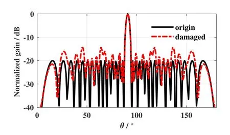
Figure 8.Display of the damaged pattern.

As an example,the 32-elements Dolph-Chebyshev antenna array is chosen to illustrate the application of AMEDO in the array failure correction.In the example,4 elements at the 3rd,8th,13rd,and 22ndpositions are defective,which cause the increase of the side lobe level.The original radiation pattern and the failure radiation pattern are shown in Fifure 8.As shown in Fifure 8,the SLL of the antenna increases from-20 dB to-14.2 dB due to the failures of the elements.AMEDO is applied to redesign the amplitudes of the excitations for the normal elements.The objective function of the optimization is to minimize the difference of the SLL of the corrected antenna array and the original array.Similar work has been done by MEDO with the corrected result of-20.003 dB,and the improved bat algorithm(IBA)with the corrected result of-20.01 dB[1,22].The corrected results of different optimization algorithms are shown in Fifure 9.The proposed AMEDO has improved the SLL from-14.2 dB to-20 dB,which is most consistent with the SLL of the original antenna array.It indicates that AMEDO can perform well in the array failure correction.

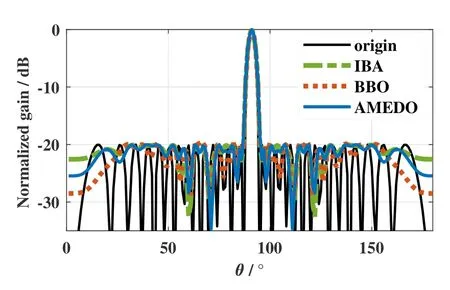
Figure 9.Comparison between the origin radiation pattern and the correction results obtained by IBA,MEDO,and AMEDO.

Table 4.Time duration of different optimization algorithms in array failure correction.

The objective function is calculated by the electromagnetic simulation software HFSS,which needs a relatively long time duration for a single calculation.In order to avoid the time cost after convergence,the optimization algorithm is terminated when the difference of the optimal solutions obtained from two consecutive calculations is less than 10-5.The calculation time durations of the different optimization methods are shown in Table 4.

The data only record the time required for the optimizations to run,without considering the workload caused by the manually adjustments of the parameters.Under the circumstance that the termination condition is the tiny difference of the two adjacent iteration results,AMEDO shows its advantage on the convergence speed.The results prove that AMEDO can greatly reduce the calculation time in the complex optimization problems,and attain a competitive solution at the same time.

VII.CONCLUSION

In this paper,the Adaptive Maxwell’s Equations Derived Optimization is proposed.AMEDO introduces the SMBO method in the iterative process of the original MEDO algorithm,and adaptively updates the parameter values.8 benchmarks are used to test the performance of the proposed AMEDO.The results show that AMEDO can achieve a matched accuracy and stability optimization result compared with the original MEDO.Because AMEDO needs no external effort to adjust the parameters,it can significantly reduce the labor cost,and avoid the degradation of the algorithm performance caused by improper parameter setting.In recent researches,agnostic Bayes provides a new way to further avoid overfitting in the parameter adaptation,which will be considered in our future studies[23,24].

ACKNOWLEDGEMENT

This work was supported by the National Nature Science Foundation of China(No.61427803).