An improved estimation of distribution algorithm for multi-compartment electric vehicle routing problem

SHEN Yindong ,PENG Liwen ,and LI Jingpeng

1.Key Laboratory of Image Processing and Intelligent Control,School of Artificial Intelligence and Automation,Huazhong University of Science and Technology,Wuhan 430074,China;2.Division of Computing Science and Mathematics,University of Stirling,Stirling FK94LA,UK

Abstract: The multi-compartment electric vehicle routing problem (EVRP) with soft time window and multiple charging types(MCEVRP-STW&MCT) is studied,in which electric multi-compartment vehicles that are environmentally friendly but need to be recharged in course of transport process,are employed.A mathematical model for this optimization problem is established with the objective of minimizing the function composed of vehicle cost,distribution cost,time window penalty cost and charging service cost.To solve the problem,an estimation of the distribution algorithm based on Lévy flight (EDA-LF) is proposed to perform a local search at each iteration to prevent the algorithm from falling into local optimum.Experimental results demonstrate that the EDA-LF algorithm can find better solutions and has stronger robustness than the basic EDA algorithm.In addition,when comparing with existing algorithms,the result shows that the EDA-LF can often get better solutions in a relatively short time when solving medium and large-scale instances.Further experiments show that using electric multi-compartment vehicles to deliver incompatible products can produce better results than using traditional fuel vehicles.

Keywords:multi-compartment vehicle routing problem,electric vehicle routing problem (EVRP),soft time window,multiple charging type,estimation of distribution algorithm (EDA),Lévy flight.

1.Introduction

The vehicle routing problem (VRP) was first developed by Dantzig and Ramser in 1959,which is a typical NPhard problem in combinatorial optimization.VRP has been studied extensively and rich research results have been achieved [1],in many of which only one type of products is considered.However,in many practical applications of VRP,more than one type of products are involved and some are incompatible.Typical examples include (i) cold chain logistics [2]with refrigerated and nonrefrigerated products,in which product deterioration and low satisfaction for customers will be caused if these two types of products are mixed together in the same compartment in the course of distribution;(ii) domestic waste collection [3]with many types of products from different recycling boxes,in which mixing all types of garbage will increase the extra workload and even lead to the failure of this recycling task;and (iii) fuel delivery [4]with multiple petroleum products,in which mixing all types of oil will directly affect the performance of oil and even cause safety accidents.Moreover,the cost will be greatly increased if all incompatible products are separately distributed by vehicles with single compartment [5].Therefore,considering the transport efficiency and cost,the capacity of a vehicle can be split into several compartments to serve different types of products simultaneously and the multi-compartment vehicle routing problem (MCVRP)is coined [6].

In addition to the above three applications,MCVRP is also applied in many other fields,such as grocery distribution [7],blood transportation [8],livestock feed distribution [9],milk collection problem [10]and so on.However,to the best of our knowledge,all research on MCVRP uses internal combustion engine vehicles,which increases the emission of greenhouse gases,pollutes the environment and consumes non-renewable energy.In recent years,government has started to take actions to reduce greenhouse gas emissions and noise levels by encouraging the adoption of electric vehicles (EVs).Many logistics companies now use EV fleets and their number is steadily increasing [11].In view of this,we attempt to apply EVs to MCVRP and make a green distribution plan for the transportation of incompatible products.Moreover,considering that the soft time window is conducive to flexible distribution [12]and multiple charging types are conducive to flexible charging to better meet the time window and reduce expenses [13],and we also take these two factors which exist in reality into our problem.At this moment,a new problem,i.e.,the multi-compartment EV routing problem with soft time window and multiple charging types (MCEVRP-STW&MCT),is proposed which uses a comprehensive objective function that minimizes the total cost of fixed vehicle cost,distribution cost,penalty cost,and charging service cost.

Compared with the basic MCVRP,when combined with the electric VRP (EVRP),the routing decisions are more challenging in presence of the practical constraints,such as soft time window constraints,multi-compartment capacity constraints,power constraints and multiple charging types considerations.Therefore,the MCEVRP-STW&MCT is a complex problem that requires innovative solution approaches.Considering that the MCVRP is an extension of the VRP and the estimation of the distribution algorithm (EDA) has a good performance in solving the VRP [14,15],in this paper we develop an EDA based on Lévy flight (EDA-LF) to solve the MCEVRP-STW&MCT.The EDA-LF algorithm performs a Lévy flight local search at each iteration to help EDA to effectively break out of the local optimum.Meanwhile,for comparison purpose,the performance is compared between the EDALF algorithm,the basic EDA algorithm without Lévy flight,and an existing algorithm.And the cost difference of the MCVRP between using EVs and traditional fuel vehicles is also compared.

The remainder of this paper is organized as follows.Section 2 reviews the relevant literature.Section 3 describes the problem and formulates the MCEVRP-STW&MCT model.Section 4 describes the concrete procedures of the proposed EDA-LF algorithm.Section 5 presents the computational experiments and the analysis on the results.Finally,conclusions are drawn in Section 6.

2.Literature survey

With the increase of application scenarios,MCVRP has gradually attracted the attention of researchers in recent years.Note that this paper studies an MCVRP combined with EVs,so we first review work on the MCVRP and then discuss the EVRP.

2.1 MCVRP

The MCVRP,which involves vehicles with different compartments for the storage of different products,is a variant of the VRP.At present,there are four kinds of popular MCVRP studies and a literature review of these different aspects is as follows.

(i) MCVRP with heterogeneous fleet

In this case,the vehicles are not exactly the same in terms of vehicle capacity,driving speed,etc.Zhang et al.used multi-compartment vehicles with different capacities and different proportions of compartments for product oil distribution,and proposed a parallel neighborhood searching algorithm of relocation and exchange operators to obtain the optimized routing scheme of vehicles [4].With the development of practical application and research,some scholars study this problem by considering flexible compartment sizes in which the size can be selected arbitrarily.Henke et al.introduced an MCVRP with flexible compartment sizes in the context of glass waste recycling in Germany in that glass of different colors should be collected separately,and a branch-and-cut algorithm was developed as the solution approach [16].

(ii) MCVRP with time windows

In this case,each customer has the requirement of service period.According to the customer’s strictness of the time window,there are two categories,depending on whether hard time windows or soft time windows are used.The former refers to the situation that the customers must be served in the time windows,and the latter refers to that the time windows can be violated if the penalty is paid.Chen and Shi studied an MCVRP with time windows for urban distribution and proposed a hybrid particle swarm optimization with simulated annealing to solve it [17].Zhan et al.established a multi-objective mathematical model for MCVRP with soft time windows and heterogeneous fleet,then proposed a variable neighborhood search algorithm for it [18].

(iii) MCVRP with split delivery

It reflects the customer’s need for multiple products that can be split separately in different vehicles.Wang et al.studied a heterogeneous fixed fleet MCVRP with split delivery in which the demand for each product must be attended in a single visit,and proposed a hybrid guided reactive tabu search algorithm to solve it [19].Furthermore,in order to split the demand more completely,Zhang et al.allowed to split delivery and each product to be delivered by multiple vehicles,and finally obtained a better distribution scheme [4].

(iv) MCVRP with stochastic factors

The stochastic factors mainly include stochastic demands or travel time.Goodson developed methods to calculate the expected time of the initial arrival to a particular customer on a priori route for the MCVRP with stochastic demands,and then described a cyclic-order simulated annealing algorithm for it [20].Lu and Wang proposed a model of clustered multi-temperature joint distribution with fuzzy travel times,and the discrete firefly algorithm is developed to solve it effectively [21].

It is important to note that the existing MCVRP with time window publications only use fuel vehicles for transportation and do not address the EVs.

2.2 EVRP

The EVRP focuses on scheduling EVs to optimize both economic and environmental costs during the distribution process.In contrast with distribution of traditional fuel vehicles,the facts that EVs are not capable of finishing a long distance due to its limited battery capacity and the number of charging stations is limited greatly increase the difficulty in solving this problem.Existing literature on EVRP often considers various factors specific to EVs,mainly including four and a literature review of these different aspects are as follows.

(i) Charging mode

At present,there are mainly six charging modes,namely slow,regular,fast charging [22],multiple charging [13],swapping battery [23],battery swaps and recharging capability which coexist in each station.Different charging modes correspond to different charging time and service price.Generally,slow charging takes 4 to 8 hours,regular charging spends 2 to 3 hours and fast charging needs 30 minutes to 1 hour [24],while swapping a new fully recharging battery takes only about 5 minutes[23]but building a battery swapping infrastructure is expensive and the battery swapping mode requires higher technology.In particular,the mode of multiple charging types provides a variety of optional charging rates and gets different recharging durations,which helps to better meet the customer’s time window and reduce energy costs.Catay and Keskin made a study firstly that extended the modeling of EVRP with hard time windows to include multiple charging options,and solved it by CPLEX.The results showed that multiple charging options may reduce the fleet size and decrease the energy costs for small-size problems such as 15 customers [25].Then,Keskin and Catay modeled the EVRP with hard time windows by allowing partial recharges with three recharging configurations which can be referred to as normal,fast and super-fast recharges,and developed a metaheuristic approach which couples the adaptive large neighborhood search approach with an exact method.The experimental results based on large-size instances and instances with tight time windows demonstrate the benefits of using multiple charging types in terms of the fleet size and the energy costs [13].

(ii) Electricity consumption

Earlier studies considered that the amount of battery discharged was either directly proportional to the distance traveled [25]or further related to vehicle load [26].Recent researches consider a comprehensive and more realistic power estimation function that includes all important parameters such as speed,acceleration,load and grade [27].

(iii) Charging time

Some studies assume that it is constant which is a plausible assumption in applications where the charging station replaces a (partially) depleted battery with a fully charged one [24].Other researchers consider that the battery level is assumed to be a linear function of the charging time [28]which is used in most researches.A few studies suggest that the actual charging function should be modeled as nonlinear [29].

(iv) Charging strategy

Firstly,according to whether partial charging is allowed,it can be divided into partial charging [30]and full charging.The former can reduce the charging time and better meet the time window,but it is more difficult to deal with.The latter is easier to solve and more concerned about charging time.Then,according to whether the charging station can be visited many times,it can be divided into single visit and multiple visits.Moreover,Desaulniers et al.[31]considered four variants of the EVRP with time windows as following and presented exact branch-price-and-cut algorithms for each:i) single full recharge;ii) multiple full recharges;iii) single partial recharge;iv) multiple partial recharges.

3.Problem description and formulation

3.1 Problem description

The MCEVRP-STW&MCT can be defined as follows.A depot has a series of homogeneous EVs.Each EV has multiple fixed size compartments.The size of the compartments can be different and each compartment is assigned to a product.A compartment must not be loaded more than its capacity.Customers have demand for different types of products which must be put into different compartments.Each customer receives service only once by a vehicle.Vehicles deliver products to customers within a given soft time windows and early or late deliveries need to be penalized.The delivery must wait until the start of the window when the vehicle arrives early.Suppose that the service time of the vehicle providing service for a customer is proportional to the customer’s demand and the ratio is 24 kg per minute.Each EV starts and ends at the depot.And as there is a restriction provided by the battery capacity,EV needs to visit the charging station nearest to the current customer point to recharge fully when it is found that the power at the next customer point is lower than the warning line for the remaining power.Since charging stations may be visited multiple times by the same vehicle or different vehicles,we create a sufficient number of copies and allow at most one visit to each.Moreover,each station is equipped with three types of charging (i.e.,slow,regular and fast charging) but only one is used at each visit to the station.The objective is to minimize the total cost,composed of fixed EV cost,distribution cost,penalty cost of violating the time window,and charging service cost.

3.2 Symbol definition

To facilitate reading,symbols related to sets,parameters and decision variables used in the MCEVRP-STW&MCT are summarized as follows.

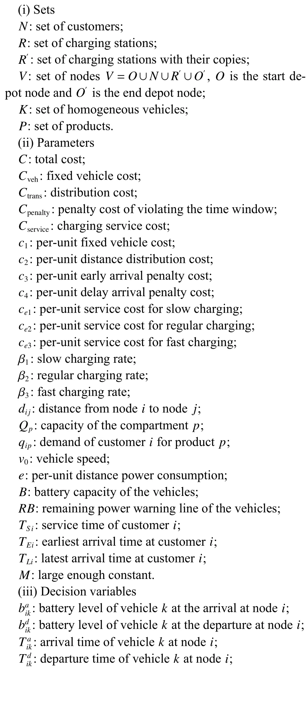
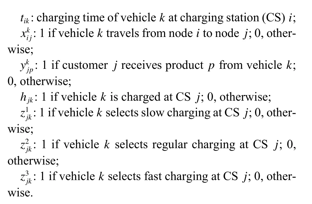
3.3 Mathematical formulation

With the above-defined symbols,the MCEVRPSTW&MCT problem can be modeled as follows:

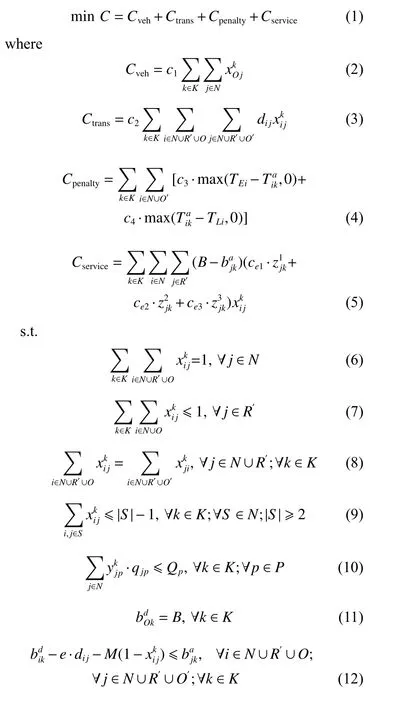
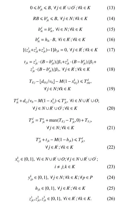
Equation (1) is the objective function that minimizes the total cost,which is composed of fixed vehicle cost,distribution cost,penalty cost,and charging service cost,as defined in (2),(3),(4) and (5) respectively.Constraint(6) ensures that each customer is visited by exactly one vehicle.Constraint (7) ensures that each charging station may be visited at most once.Constraint (8) ensures the continuity of each route.Constraint (9) is a classical subtour elimination constraint.Constraint (10) states that a compartment must not be loaded more than its capacity.Constraint (11) ensures that vehicles depart from the depot with full battery.Constraint (12) represents the change of battery power after the vehicle successively visits two nodes.Constraint (13) ensures that the vehicle has enough power to reach the charging station or return to the end depot.Constraint (14) requires that the power of the vehicle when it reaches the customer node must be greater than the remaining power warning line.Constraint (15) states that the power of vehicle remains unchanged before and after visiting the customer node.Constraint (16) indicates that the battery is fully charged if the vehicle visits the charging station.Constraint (17)states that only one charging type can be selected if the charging station is visited.Constraint (18) represents the charging time of the vehicle at the charging station.Constraint (19) is the departure time of each vehicle from the start depot.Constraint (20) represents the arrival time of the vehicle at the next node.Constraint (21) presents the departure time of the vehicle after serving the customer node.Constraint (22) represents the departure time of the vehicle after charging at the charging station node.Finally,constraints (23) − (26) define the 0-1 decision variables.

4.EDA-LF for MCEVRP

In this section,the EDA-LF for solving the MCEVRPSTW&MCT is presented in details.First,the encoding and decoding schemes,probability model and sampling process,adaptive updating mechanism,and local search based on Lévy flight are proposed.Then,the flowchart of the EDA-LF is provided.

4.1 Encoding and decoding schemes

Every individual of the population denotes a solution of the MCEVRP-STW&MCT,which is represented by a sequence of all the customer numbers.The sequence decides the order of delivering products to customers.This solution representation has been widely used in the VRPs[32].

Decoding a sequence is to arrange the vehicles to serve all the customers which need multiple incompatible products and determine the charging plan for each vehicle,so as to generate a feasible schedule.In particular,for the charging plan,in addition to timely arranging the nearby charging stations for charging,it is also necessary to flexibly select the appropriate charging type according to the tightness of the next arrival node’s time window.According to the constraints of MCEVRP-STW&MCT and human experiences,we design an effective decoding scheme and the specific steps are as follows.

Step 1Select the maximum value of the power consumption of all customers to their nearest charging station,and round up this value as the remaining power warning lineRB.

Step 2Insert depot node 0 at the beginning and end of the encoding sequence.Then,check the customer sequence from front to back and if compartment capacity is exceeded at a customer point,then insert two depot nodes 0 before that customer point.After that,all customers are assigned to theHvehicles numbered {1,2,3,···,H},namelywherexhjmeans the number of thejth customer to be served on the vehiclehandKhis the total number of customers served by vehicleh.Seth=1.

Step 3Ifhis greater thanH,go to Step 9;otherwise,go to Step 4.

Step 4Set the departure time of vehiclehleaved f rom start depot 0 by calculating the time

Step 5If the remaining power calculated by constraint (12) at the (j+1)th customer node is greater thanRBafter the vehicle has served itsjth customer,then go to Step 6;otherwise,charge at the charging station nearest to thejth customer node and set the mark flag=0,then go to Step 7.

Step 6Setj=j+1 and ifjKh,then go to Step 5;ifj=Khand the current remaining power is not enough to return to end depot 0,then charge at the charging station nearest to thejth customer node and set flag=1,then go to Step 7;otherwise,go to Step 8.

Step 7Select the charging type with the lowest total cost among the three charging types for the nearest charging station which is obtained by comparing the cost(namely the sum of the charging service cost corresponding to the charging type and the penalty cost of the time window at the next arrival node) of each charging type.If flag=0,then go to Step 6;otherwise,go to Step 8.

Step 8Seth=h+1 and go to Step 3.

Step 9End.

To better understand this decoding process,an example is given in Fig.1 wherenandmrespectively represent the quantity of customers and charging stations whose numbers aren+1 ton+m,and Ⅰ,Ⅱ and Ⅲ respectively represent the three charging types of slow,regular and fast charging.For the individual that the customer sequence is encoded as [1,2,3,···,n−1,n],its decoding process is shown in Fig.1.After getting the distribution scheme by the above decoding process,the objective function in the mathematical model is used as the fitness function to evaluate the individual.

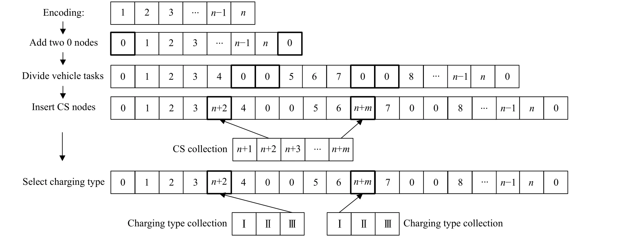
Fig.1 Schematic diagram of the decoding process

4.2 Probability model and sampling process

Different from the genetic algorithm (GA) that produces offspring through crossover and mutation operators,the EDA does it by sampling according to a probability model [33].Thus,the probability model has a great effect on the performance of the EDA.In this paper,to well reflect the property of the considered problem,the probability model is designed as a probability matrixP(g) as follows:

The elementpij(g) of the probability matrixP(g) represents the probability that customerjappears in positioniof the solution sequence at generationg.The value ofpij(g) refers to the importance of a customer when deciding the scheduling order.For all values ofiandj,pij(0) is initialized topij(0)=1/n,which ensures that the whole solution space can be sampled uniformly.

In each generation of the EDA,the new individuals are generated via sampling the solution space according to the probability matrixP(g).For every positioni,customerjis selected by the roulette-wheel method according to theith row of the probability matrixP(g).If customerjhas already appeared,it means that customerjhas been scheduled.Then,the wholejth column of probability matrixP(g) will be set as zero and all the elements ofP(g) will be normalized to maintain that each row sums up to 1.In such a way,an individual is constructed until all the customers appear in the sequence,and then its fitness value can be calculated.

According to this sampling strategy,in our EDA,the initial population can be generated by samplingP−size times while the other generation population in the subsequent iteration process is composed of (1−b%)×P−size sampling individuals and the bestb%×P−size elite individuals of the previous generation population,wherebrepresents the percentage of the population retained from the previous generation.

4.3 Adaptive updating mechanism

In addition to the sampling way based on the probability model,only by updating the probability model reasonably,the EDA-LF could trace the more promising search area.At each generation,the probability matrix is updated by the information of some elite solutions of the population.The elite sub-population consists of the bestSP−size solutions,whereSP−size=η%×P−size and η is the percentage of elite individuals in the population.To be specific,the updating process can be regarded as the following incremental learning [33]:

In addition,α(g) is the learning rate of the probability matrixP(g) at thegth generation.To speed up convergence,the adaptive learning rate [34]is adopted as follows:

where α(0) is the initial learning rate.In such a way,the learning rate may be relatively large at the earlier period of the search process to accelerate the speed of convergence.As the population evolves,the learning rates decrease exponentially so as to enhance the exploitation ability.To ensure certain learning efficiency,we set the l earning rate no less than 0.01 for the above equations.

4.4 Local search strategy based on Lévy flight

The EDA pays more attention to global exploration while its exploitation capability is relatively limited,which makes it easy to premature convergence and fall into local optimum.Thus,an effective EDA should balance the exploration and the exploitation abilities.Therefore,in this paper,a Lévy flight search is introduced into EDA to enhance its local exploitation around the best solution of the current population several times at every generation.

The Lévy flight search is an alternate way of walking with a short distance search combined with occasional longer distance walking [35],which is a random search path and it obeys a Lévy distribution [36],that is a probability distribution proposed by the French mathematician Lévy in the 1930s.Lévy flight can increase the diversity of the population and broaden the scope of the search,which makes it easier to jump out of local optimal points in the intelligent optimization algorithm such as firefly algorithms [37]and cuckoo search [38].

The Lévy flight location update formula is as follows:

Due to the complexity of Lévy distribution,it is usually simulated by the Mantegna algorithm and the step sizesis calculated as follows:

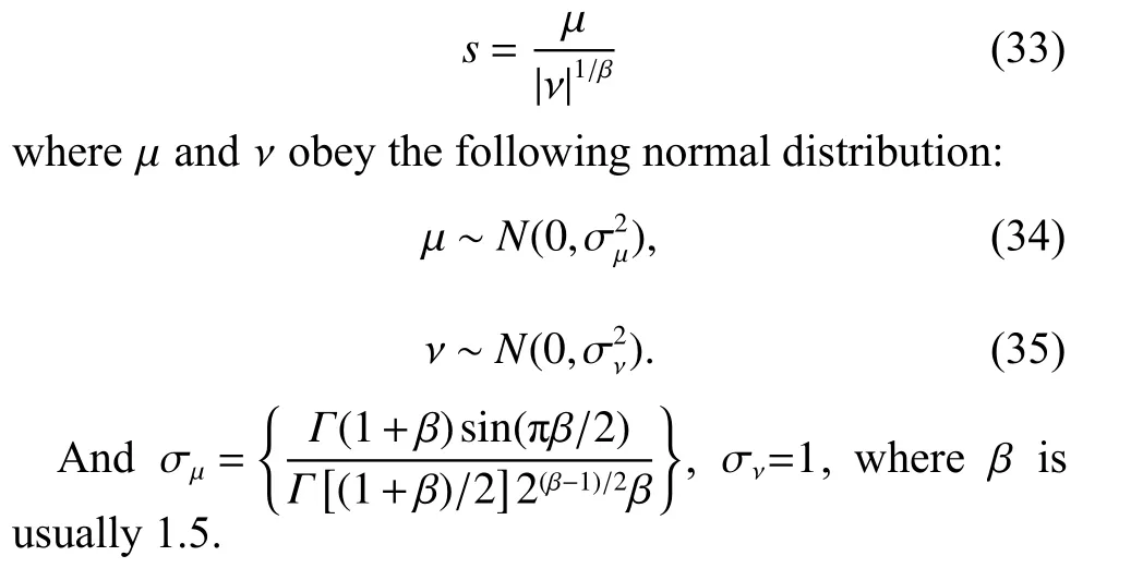
It should be noted that the new solutionobtained by updating the current optimal solution through the Lévy flight search is a vector with continuous values,while the natural number encoding is used as solution representation in this paper and it is discrete.Therefore,it is necessary to construct a proper mapping from a vector with continuous values to non-repeated natural number permutation.For this,the rule based on ranked order value(ROV) in [39]is adopted to convert the continuous value of each position in the solution sequence into the discrete customer number after ranking according to the ROV rule to form a feasible solution.

In order to better understand the whole process of Lévy flight local search,an example is given in Fig.2 below.

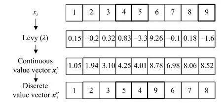
Fig.2 Schematic diagram of Lévy flight local search

From Fig.2,it can be found that the whole process of Lévy flight local search is similar to the exchange or insertion operation,or even the combination of these two neighborhood searches.That is,the change from[1,2,3,4,5,6,7,8,9]tounderstood as the exchange of customer 4 and customer 5 firstly and then inserting customer 9 before customer 6.

Moreover,in order to improve the possibility of improving the solution quality of the EDA algorithm in the local search process,it is necessary to use Lévy flight operation multiple times on the best individual of the current population at every generation.In general,the solution quality is easy to be improved at the earlier period of the search process while it becomes more and more difficult as the population evolves into the middle and later periods.Therefore,in order to save the running time of EDA and ensure the ability to jump out of the local optimum at the middle and later periods,we set the number of Lévy flight local search as in the following logistic curve:

which is related to iteration numbertand this curve is fitted by Matlab.After that,if the fitness value of the optimal individual obtained by multiple Lévy flight search is smaller than the best individual of the current population,then use the former to replace the latter.

4.5 Algorithm flowchart

With the above design,the flowchart of the EDA-LF for solving the MCEVRP-STW&MCT is illustrated in Fig.3.

At the initial stage of the evolution process,the whole search space is sampled uniformly.Then,the algorithm uses the EDA-based evolutionary search mechanism to sample a potential area.In addition,the local search based on Lévy flight is implemented in a promising region,aiming to obtain better solutions.With the benefit of combining EDA and Lévy flight local search,global exploration and local exploitation are balanced.In this paper,the stopping condition is that the maximum number of generations reaches 200.

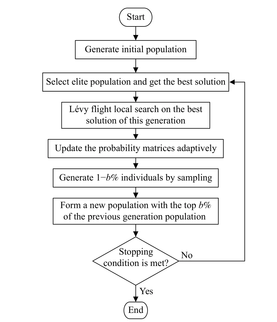
Fig.3 Flowchart of the EDA-LF

5.Computational experiments

To investigate the performance of the proposed EDA-LF approach for MCEVRP-STW&MCT,we implement the algorithm using Microsoft Visual Studio 2013.A computer with Intel (R) Core (TM) i5-8250U CPU is adopted to run the code for all instances,and the operating system is Windows 10.We generate the MCEVRP-STW&MCT instances and set the model parameters according to the existing literature firstly,then compare the performance of the EDA-LF,basic EDA (BEDA),and an existing algorithm,and finally compare the cost difference of the MCVRP scheme between using EVs and traditional fuel vehicles.

5.1 Test instances and model parameters

Since there are no internationally recognized instances for MCEVRP-STW&MCT,we adopt the method proposed in [40]to generate the MCEVRP-STW&MCT instances based on the VRP with time windows (VRPTW) instances of Solomon [41].Those VRPTW instances have three set instances involving 25,50 and 100 customers respectively.According to the customer position distribution,instances of each set are divided into clustered distribution C classes,scattered distribution R classes,and partial scattered and partial clustered distribution RC classes.In addition,considering the limited space,we only consider the narrower time window“1”classes rather than the wider time window“2”classes.In consequence,Solomon’s instances used in this paper are subdivided into three classes,C1,R1 and RC1.Then,those VRPTW instances are adapted into MCEVRP-STW&MCT instances according to the method proposed by Reed [40],in which the data is obtained by dividing the vehicle capacity into two compartments in a ratio 3:1,and the customer demands are also divided by using a 3:1 ratio except the demands of the sub-regionwhich are divided using a 2:1 ratio.In the representation of the sub-region,xandyare the horizontal and vertical coordinates of the customer position,xmaxandymaxdenote the maxima of the horizontal and vertical coordinates,xminandymindenote the minima of the horizontal and vertical coordinates.

In addition to setting the customers information as above,the location of the charging station should also be given.It is assumed that three set instances involving 25,50 and 100 customers correspond to 5,10 and 20 charging stations respectively,and these charging stations are uniformly distributed in a 100×100 area.Finally,some fixed parameters of the MCEVRP-STW&MCT model are set in Table 1 in which most of the them are set by existing literature while a few are set in the paper.

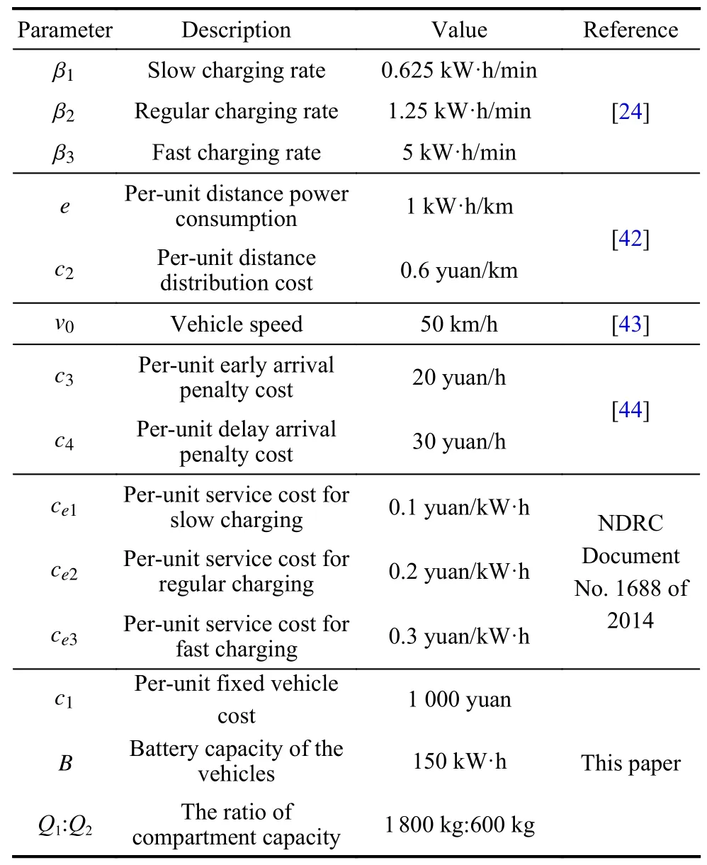
Table 1 Model parameter setting

5.2 Parameters setting of EDA-LF algorithms

The proposed EDA-LF algorithm has four key parameters to be set:P−size (population size),η (percentage of elite solutions),the initial learning rate α(0),andb(percentage of remaining elite individuals of the previous generation).To investigate the influence of these parameters on the performance of the EDA-LF,and explore whether different customer sizes or customer distribution types lead to differences in parameters setting,the Taguchi method of design-of-experiment (DOE) is implemented by using the first instances of each class with different customer sizes in Solomon’s instances.Due to the limited space,only the specific DOE process of C101 instance with 25 customers is shown here.Combinations of different values of these parameters are listed in Table 2.

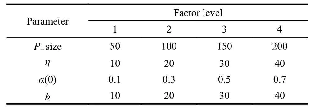
Table 2 Combinations of parameter values

According to the number of parameters and the number of factor levels,we choose the orthogonal arrayL16(44).For each parameter combination,the EDA-LF is run 10 times independently and the average fitness value obtained by the EDA-LF is calculated as the response variable (RV) value.The orthogonal array and the obtained RV values are listed in Table 3.

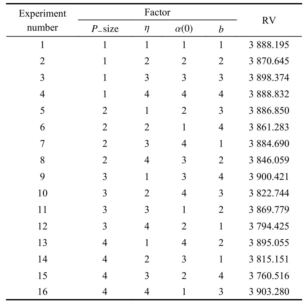
Table 3 Orthogonal array and RV values

According to the orthogonal table,we figure out the average RV(ARV) values of each parameter to analyze its significance rank which is listed in Table 4.Then,the influence trend of each parameter is illustrated in Fig.4.

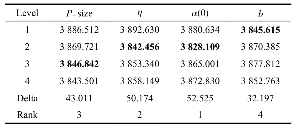
Table 4 ARV and rank of each parameter

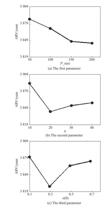
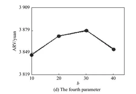
Fig.4 Influence trend of each parameter

From Table 4,it can be seen that the initial learning rate α(0) is the most significant one among the four parameters.This means that the initial learning rate is crucial to the performance of the EDA-LF.A small value of α(0)could lead to slow convergence while a large value could lead to premature convergence.Therefore,to ensure the effectiveness of the EDA-LF,an appropriate value of α(0) is very essential.In addition,η ranks the second.A proper value is helpful to update the probability model efficiently.Besides,the significant rank of the population size is the third.A large value ofP−size makes the algorithm sample the solution space sufficiently but it will cause a large amount of computational budget.It can be seen from Fig.4 that it makes no significant improvement when the size is too large.In this case,to reduce the computational budget,we setP−size=150.Finally,although parameterbhas the slightest influence,adding some elite individuals of the previous generation to the current population will help the algorithm converge and further optimize.According to the above analysis,a good choice of parameter combination is suggested asP−size=150,η=20,α(0)=0.3,b=10.

In order to explore whether different customer sizes or customer distribution types have an impact on the parameters setting,the DOE method is further used to other eight instances numbered 101.Finally,these nine DOE results are summarized in Table 5.

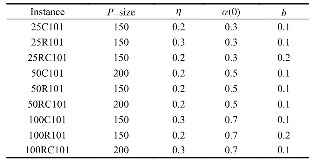
Table 5 Summary of nine DOE results

From Table 5,it can be found that the initial learning rate α(0) gradually increases with the problem scale,while other obvious rules or conclusions have not been found yet.This is because that the solution space increases greatly with the problem scale,the initial learning rate α(0) also needs to be increased to make the algorithm converge quickly at the earlier period to get closer to the optimal solution which can achieve a better optimization effect.The results of the above algorithm parameter setting will be further applied to the following experiments.

5.3 Comparison of EDA-LF and BEDA

In order to verify the effectiveness of adding the Lévy flight local search strategy to the EDA algorithm,we still use the nine instances (i.e.,the first instances of each class with different customer sizes in Solomon’s instances)to compare the performance of EDA-LF and BEDA without Lévy flight local search.The two algorithms use the same parameter setting for each instance and the maximum number of iterations is 200.After that,we can find that for the small,medium,large-scale instances (i.e.,corresponding to 25,50 and 100 customers,respectively),the computational times are 46 s,77 s and 198 s respectively,which are within an acceptable time range.Also,for each instance,we can get the best value,the mean value and the standard deviation that are achieved by running two algorithms 10 times independently,and the results are shown in Fig.5,Fig.6 and Fig.7 respectively.

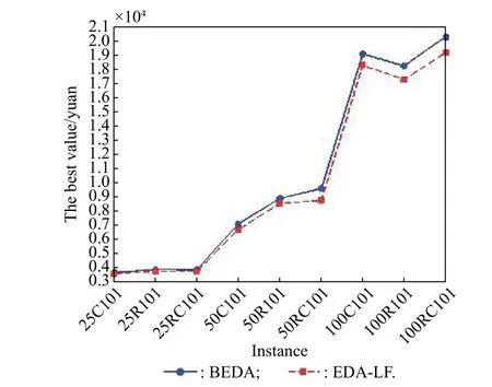
Fig.5 Comparison between BEDA and EDA-LF for the best value

From Fig.5 and Fig.6,we can see that the curves of EDA-LF are all below BEDA which indicates that the optimal value and average value found by the EDA-LF algorithm are better than those by BEDA.Therefore,the EDA-LF algorithm can find a better solution and the Lévy flight strategy is effective for solving the MCEVRPSTW&MCT.In addition,it can be seen from Fig.7 that the standard deviations of the EDA-LF are all smaller than those of the BEDA.Accordingly,we conclude that the EDA-LF is more robust than the BEDA.

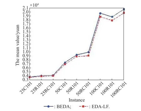
Fig.6 Comparison between BEDA and EDA-LF for the mean value

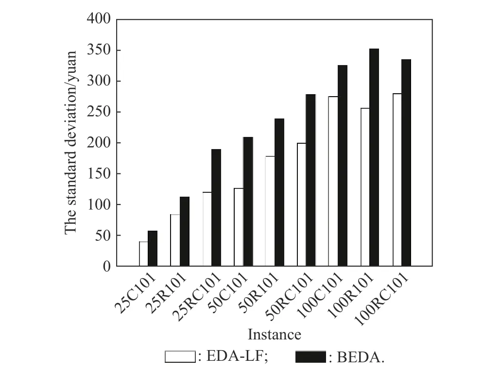
Fig.7 Comparison between BEDA and EDA-LF for the standard deviation

5.4 Comparison with an existing algorithm

Next,the EDA-LF is compared with the GA [45]which is proposed to solve the MCVRP with flexible compartment sizes by Koch et al.Moreover,to compare the performance of these two algorithms fairly,we all set the stopping criterion of 100 s,which is an acceptable short time.The parameters of the GA are set as follows:the crossover probabilityPco=0.9,the probability in the swap mutation operatorPswap=0.05 and the probability in the inversion mutation operatorPinv=0.05.The parameters of the EDA-LF are set as in Table 5.For each of these 27 instances,the EDA-LF and the GA are used to solve the MCEVRP-STW&MCT and run 10 times independently,then the mean values are listed and the differe nce values ∆E−Gare calculated in Table 6.

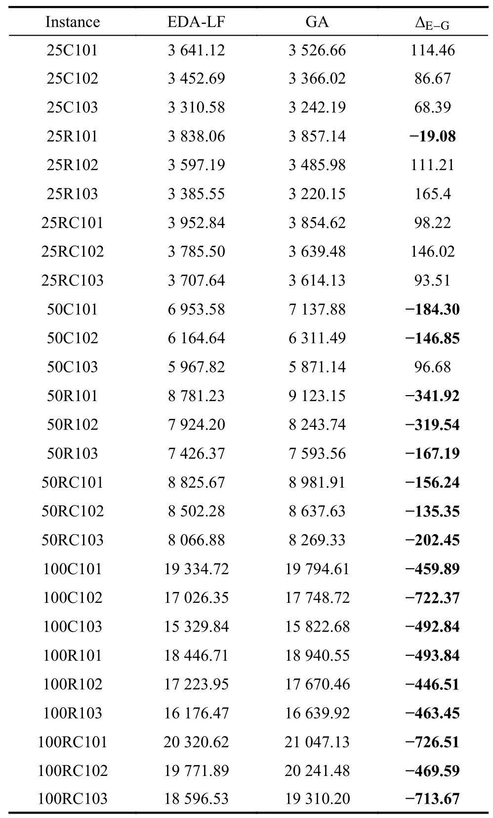
Table 6 Comparison between the EDA-LF and the GA

From Table 6,it can be seen that the EDA-LF outperforms the GA in 18 instances,whose difference value is negative and bold.And we can also find that the EDA-LF is better than the GA for the medium and large-scale instances except for instance 50C103,while worse than the GA for the small-scale instances except for the instance 25R101.Therefore,in general,compared with the GA,the EDA-LF can often get better solutions in a relatively short time when solving medium and large-scale instances.

5.5 Comparison in MCVRP between using EVs and traditional fuel vehicles

The existing researches on MCVRP usually use the traditional fuel vehicles to transport incompatible products.In order to discuss the difference of MCVRP between using EVs and traditional fuel vehicles,we use the proposed EDA-LF algorithm to solve the multi-compartment fuel vehicle routing problem (MCFVRP),in which the compartment capacity of a traditional fuel vehicle is the same as that of an EV in MCEVRP.Considering that there are many fuel stations and the refueling time is short,we ignore the refueling time in MCFVRP and set the per-unit distance distribution cost of the traditional fuel vehicle to 1.5 yuan according to [46].For simplicity,only these 27 instances (i.e.,the first three instances of each class with different customer sizes in Solomon’s instances) are used and the mean value is achieved by running the EDA-LF algorithm 10 times independently.Finally,the relative percentage deviation (RPD,RPD=(E−F)/F·100%) between the mean value of MCEVRP and the MCFVRP is calculated,and the results are shown in Table 7.

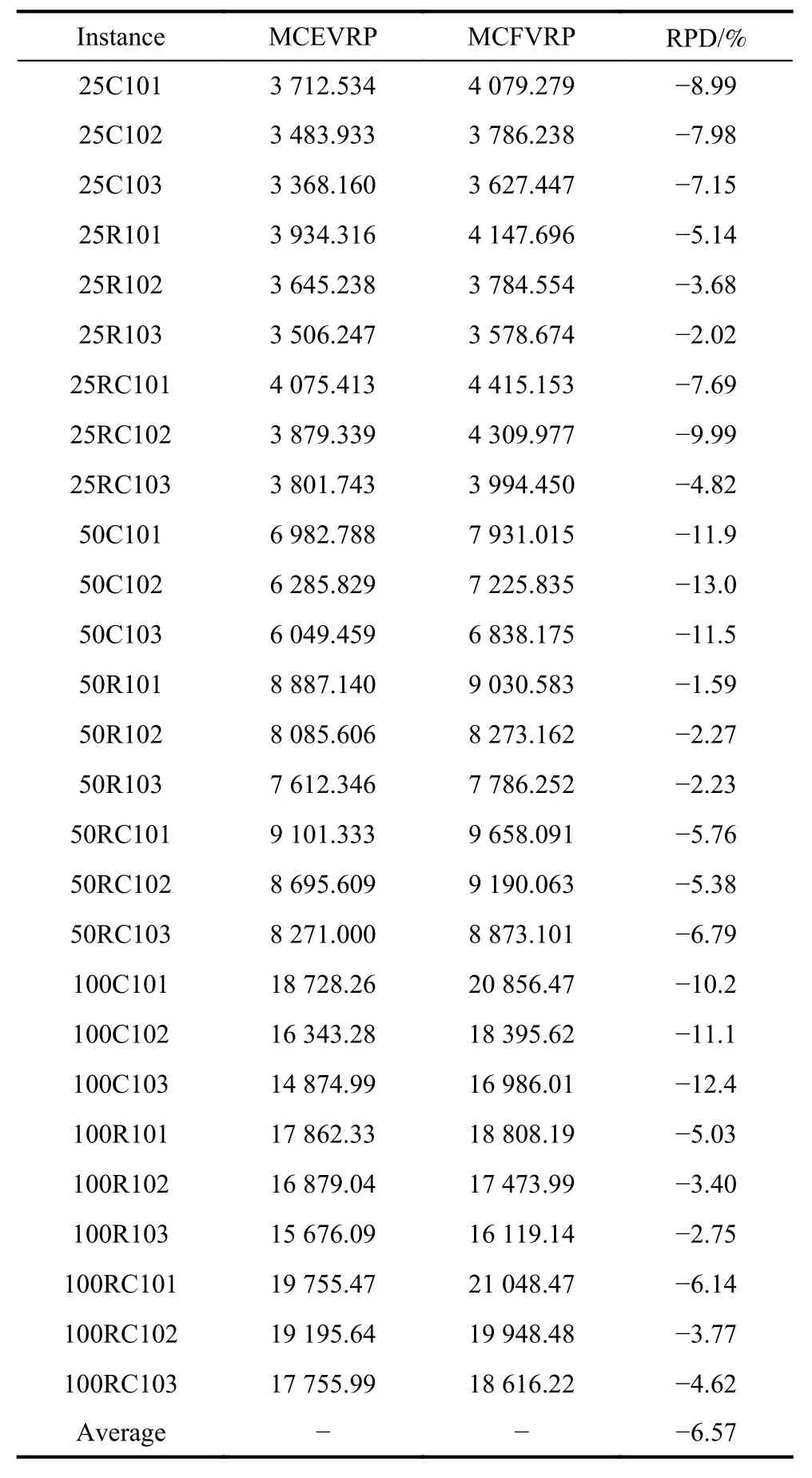
Table 7 Comparison of EDA-LF solutions for MCE VRP and MCFVRP

From the 27 rows of data in Table 7,it can be seen that the cost of MCEVRP using EVs is all less than that of MCFVRP using traditional fuel vehicles and the distribution cost of using EVs can be reduced by 6.57% on average.This shows that although the distribution mode of using EV will increase the charging service cost and its longer charging time may lead to higher penalty cost of the time window under the flexible choice of various charging types,it has a lower energy consumption compared with the distribution mode of using the traditional fuel vehicle which greatly reduces the distribution cost.Moreover,with the increase of punishment on exhaust emissions of fuel vehicles and considerable subsidy policy for distribution of EVs,the cost of MCEVRP will be further lower than that of MCFVRP.More importantly,the use of EVs has less pollution to the environment and helps to reduce greenhouse gas emissions.

Therefore,using multi-compartment EVs to transport incompatible products can not only reduce costs,but also protect the environment which makes it more attractive to logistics companies and more popular with the public than using traditional multi-compartment fuel vehicles.In addition,the multi-compartment EV distribution scheme developed in this paper will be helpful to guide the green logistics distribution of incompatible products.

6.Conclusions

In this paper,the MCEVRP-STW&MCT is proposed,which is a combination of the MCVRP and the EVRP.After constructing the mathematical model of the problem,an EDA-LF is proposed,in which a specific decoding scheme is devised whilst a Lévy flight local search is employed to help the EDA algorithm jump out of the local optimum.Experiments for comparing the EDA-LF and the BEDA have been conducted,in which the DOE method is used to set the algorithm parameters.The results show that the EDA-LF algorithm can not only find a better solution,but also has a stronger robustness compared with the BEDA.In addition,when comparing with existing algorithms,the result shows that the EDA-LF can often get better solutions in a relatively short time when solving medium and large-scale instances.Furthermore,we use the proposed EDA-LF algorithm to solve the MCFVRP,and discuss the cost difference of MCVRP between using EVs and traditional fuel vehicles.In addition to protecting the environment,the result shows that the cost of using electric multi-compartment vehicles to distribute incompatible products is lower than that of using traditional multi-compartment fuel vehicles.

With the requirements of green logistics and the increase of distribution demand of incompatible products,the multi-compartment EV distribution scheme proposed in this paper will be helpful to provide guidance for the distribution of incompatible products.Moreover,it is also helpful to promote the establishment of a low-carbon and low-pollution distribution system.