
Research of aerodynam ic characteristics of heavy commercial vehicles under crosswind for different urban road layout
2020-12-23 05:15:48SongLIJinchengLIChunboDONGTianhongLITengfeiLIYuanhangSHENWeiYANJingyuWANGXingjunHU
机床与液压 2020年18期
Song LI,Jin-cheng LI,Chun-bo DONG,Tian-hong LI,Teng-fei LI,Yuan-hang SHEN,Wei YAN,Jing-yu WANG*,Xing-jun HU
(1 School of Aviation Operations and Services,Air Force Aviation University,Changchun 130022,China)
(2 College of Automative Engineering,Jilin University,Changchun 130022,China)
Abstract:Based on the dynamic meshing technology,and adopting the partial joints displacementmode,the transient aerodynamic characteristics of three schemes that the heavy commercial vehicle passing the leeward side of single building,passing the windward side of single building and passing thewindward side of double buildings about urban roadswere studied.The displacement velocity of themesh joint,namely the driving velocity of heavy commercial vehicle,was set at15 m/s,and the velocity of the crosswind was 10 m/s.The results show that the effects of buildings on the transientaerodynamic characteristics are relatively obvious.During the driving,the change values of lateral force coefficient and yawingmoment coefficient can be up tomore than 5.0 in one second.And the corresponding change values of lateral force and yawing moment are about 12 kN and 30 kN·m,which make the peak change rates of lateral force and yawingmoment reach to-12 kN·s-1 and 35 kN·m·s-1.In addition,the direction of these two parameters have changed twice during the driving process.
Key words:Heavy commercial vehicle,Crosswind,Dynamicmesh,Urban road,Transient aerodynamic characteristics
1 Introduction
The aerodynamic characteristics of vehicle are important aspect of the whole vehicle performance,which are closely related to the driving safety and stability[1].In the process of driving,the air flow around the vehicle is turbulent.The velocity and its direction of the air flow change with time,being of transient characteristics[2].Due to the complicated urban road configurations,natural or artificial gusts are likely to occur and threat the driving safety.In order to avoid the problems caused by the gusts,heavy commercial vehicles are required to have good aerodynamic characteristics under crosswind conditions[3-4].Previous studies on crosswind conditions have usually been carried outwhen the vehicles are crossing bridges or tunnels[5-8],but few studies have been conducted on crosswind caused by urban buildings,which is a very common operating condition.There-fore,the aerodynamic characteristics of heavy commercial vehicles under crosswind formed by different urban buildings are studied in this paper.
The numerical simulation is applied to heavy commercial vehicles by using the CFD software FLUENT,dynamic meshing technology and SST k-ωturbulence model.The three operating conditions are the heavy commercial vehicle passing the leeward side of single building,passing the windward side of single building and passing the windward side of double buildings respectively.Through thismethod,the transient aerodynamic characteristics,the changing law of aerodynamic load and its distribution of the heavy commercial vehicle in different urban road environment are obtained.This work provides theoretical basis for the driving safety under urban road condition.
2 Calcu lation model
2.1 Geometricmodel of heavy commercial vehicle
Fig.1 shows the size of thewhole heavy commercial vehiclemodel.It is provided by a domestic car factory.Themodel is a combination structure of tractor and semi-trailer.The length of the whole vehicle,reaches 14.2m including the container,the height is 3.75 m and themaximum width is 2.5 m.There is a 1.3 m wide gap between the tractor and the trailer.The front view of themodel is shown on the left side of Fig.1,while on the right side of the figure is the side view from the driver’s right perspective.
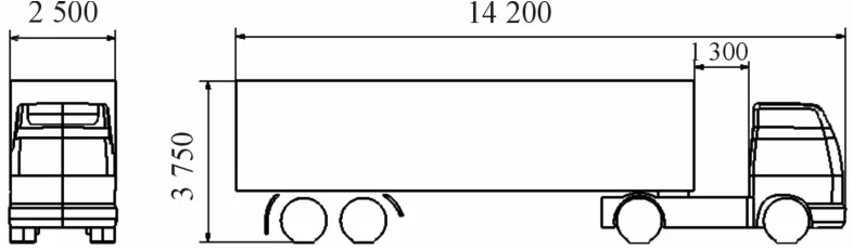
Fig.1 The size of the heavy comm ercia Ivehic Ie(mm)
2.2 Building model and its layout
This paper adopts the common office building as the basic architectural form.The geometric model of the building is shown in Fig.2.According to the Industry Standard of the People’s Republic of China[9],the model in Fig.2 is a 5-storey office building.The attic structure above the top floor is 2m high,with a total height of 17m.The width of the building is set at 8m and the length is set at2 times of the car body to ensure a stable flow field before the vehicle entering the gust boundary and exiting it.The windows and other structures of actual office buildings are ignored here.

Fig.2 The sim p Iified m ode Iof sing Ie buiIding and its size(m)
Three different layouts of building are shown in Fig.3.In the figure,Vwis the crosswind speed,andVcis the speed of heavy commercial vehicles.Layout 1indicates that heavy commercial vehicles are located on the upward side of a single building.Layout 2 shows that heavy commercial vehicles are on the downwind side of single building.Layout3 is the situation that heavy commercial vehicles are located on the downwind side of two tandem buildings.
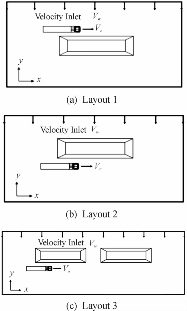
Fig.3 Three different schematic of buiIding Iayout
2.3 Size of the road
The distance between the heavy commercial vehicle and the building in this scheme is determined by the road width.According to the Industry Standard of the People’s Republic of China[10],three two-way road configurations are adopted and assuming that there are only sidewalks between buildings and highways.In the simulationmodel,the road configuration is simplified as a single road with three parallel lanes.Each lane is5m wide.And,the totalwidth is15m.There are sidewalks and curb belts on the two sides of the driveway.Both the sidewalk and the belt are 3 m wide.The schematic diagram of road size is shown in Fig.4.
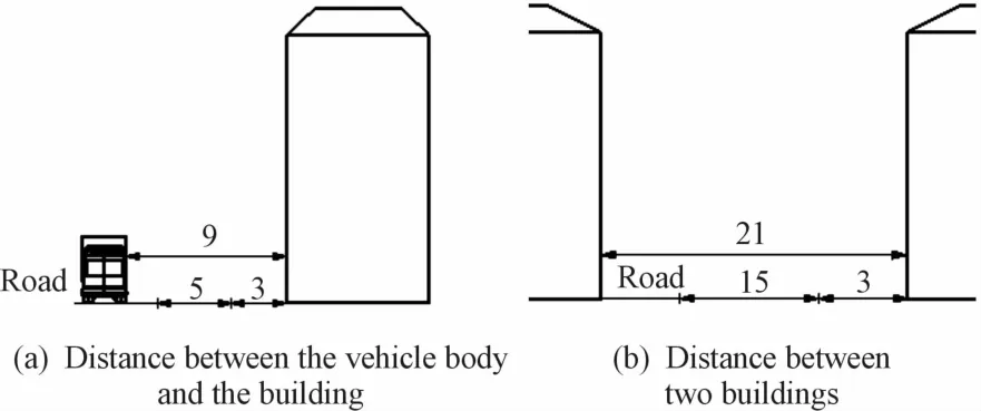
Fig.4 The schem atic of the road size(m)
3 Num erical sim u lation schem e
3.1 Dynamicmessing theory
In the dynamic messing method,the displacement of the grid is closer to the actualmotion,and thus the accuracy of the simulated numerical flow field obtained by calculation is greater than the real physical one.Therefore,in this paper,the dynamic messing technology is applied to simulate the transient characteristics of the flow field.
Hexahedral structure is applied to the dynamic messing.And the displacement of the grid is realized bymerging or squeezing themesh whose size exceeds a certain critical value according to the dynamic laying-overmethod.Consequently,the real-time update of grid coordinates is finished.The core idea of the dynamic layer-over model is that adding or reducing the dynamic layer with the change of the height of the layer adjacent to the moving boundary[7].In other words,when the height of the grid layer adjacent to themoving boundary increases to a certain value,the layer is divided into two grid layers.If the height is reduced to a certain extent,the two adjacent mesh layers aremerged into one layer,as shown in Fig.5.In Fig.5,i and j represent the grid in layer i,j near themoving boundary.When the boundary moves upward,themesh is compressed and the height h of the mesh in layer j gradually decreases.When the height is less than a critical value,layer j ismerged into layer i and a new layer i is formed with a height ofh+hideal.At this time

Where,αcis called merging factor,andhidealis the ideal grid height.If the boundarymoves downward and stretches the grid,the height of the grid on layer j gradually increases until

Where,αsis called segmentation factor.In this case,the grid on layerjwill be split into two layers,layerjand layerj+1,with height ofhidealandh-hideal,respectively.So,it can be seen that the dynamic layerovermethod is to realize the displacement of moving boundarymessing bymerging or splitting the grid.

Fig.5 The p rincip Ie of the m esh re Iocation for dynamic Iayer sp read m ethod
Because the overall displacement of the grid is hindered by the buildings in urban roads,the moving mode of local node displacement are adopted in this paper.
3.2 Division of computational domain
Fig.6 is a schematic diagram of the calculation domain of the first building layout.The width of upwind side and downwind side in the calculation field are 10 times and 3 times the vehicle length,respectively.At the beginning,the distance from the head of vehicle to the building is 1.5 times the vehicle length,and the total driving distance is 84m.In order to improve the calculation efficiency,the initial distance from the rear part of the body to the boundary of the computational domain is 1 time the vehicle length and 7 times the vehicle length from the front part.
The width of the upwind side of the second type of building layout is set to 4 times the vehicle length to ensure that there is enough space to arrange the grid on the upwind side.While the downwind side of the calculation area is 9 times the vehicle length.The remaining dimensions are the same as the first layout.
In the third layout,another building with an interval of21m is added on the basis of the second layout.The distance between the front of the vehicle to the boundary of the calculation field in the initial state is increased to 11 times the vehicle length,and the driving distance reaches 133 m.The other dimensions are the same as the second layout.
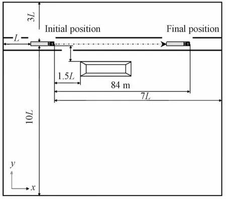
Fig.6 The size of the com putationa I dom ain for the first buiIding Iayout
3.3 Boundary conditions and solution settings
The inlet and the outlet are set as the velocity inlet and the pressure outlet,respectively.The front and rear surfaces and the top surfaces are set as the symmetrical surfaces.The channel boundary is set as the interface surface.Suppose the ground and the body surface are non-sliding wall surfaces,where the ground is the fixed wall surface and the body surface is themoving wall with a speed of 15 m/s along the positive direction ofx-axis.
The total driving time is5.6 s,5.6 s and 8.9 s respectively in the three building layouts.In this scheme,the time step is 0.001 s.Therefore,the number of time steps in each layout is 5 600,5 600 and 8 900 respectively.
SSTk-ωmodel was selected for turbulent flow field.The Standard discrete format is only applied to pressure,the other physical quantitieswere in the second-order upwind discrete format,and the first-order implicit discrete scheme is used for time variable.
3.4 Arrangement of observation points
In order to ensure that the selected observation points can fully reflect the changing law of transient aerodynamic characteristics,observation points are arranged according to the time of the vehicle bodymovement in this paper.From the beginning ofmovement,one observation point is set up every 0.1 s,which is 100 time-steps.During the calculation,only when the head of vehiclemoves to the observation pointwill the calculated results be outputand saved into a data file.Therefore,there are 56,56 and 89 observation points in the three different building layouts,as shown in Fig.7.When the heavy commercial vehicle starts to enter or leave the building area,themovement time is about1.4 s,3.2 s,4.5 s and 6.5 s.Therefore,the position is indicated by the head reaching the observation points14,32,46 and 65.In the figure,the horizontal axis is motion time t,namely the observation point.The vertical axis is the physical variable such as the aerodynamic coefficient,etc.,denoted byφ.Fig.7 shows the third layout.The observation points of the other two layouts are the same as the first half of the figure and end at point56.
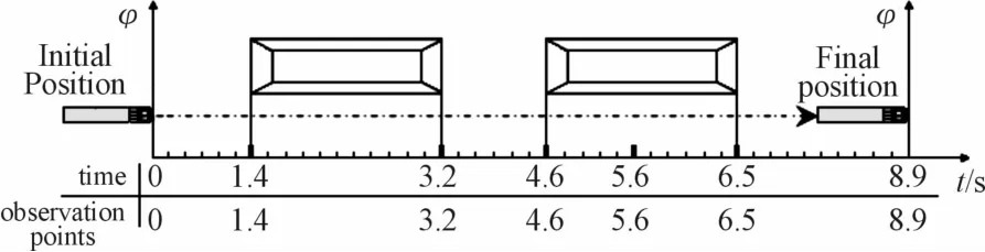
Fig.7 The schem atic of the reIationship of the observation point and m oving time
4 Analysis of transient simulation results
4.1 Variation law of aerodynamic force coefficient and moment coefficient
4.1.1 Analysis of aerodynamic resistance coefficient
Fig.8 shows the changing law of the resistance coefficientwith time under three different forms of building layout.It can be observed that variation of the transient aerodynamic characteristics of the heavy commercial vehicle.TheCDvalues for the first two layouts rises slightly to about1.7 beforet=1.0 s.After that,the resistance coefficients began to decline.Comparatively,it decreases faster in the second layout and down to about0.6,and then begins to rise att=1.8 s.Meanwhile,the resistance coefficient for the first layout still decreases.At this stage,the car body reaches and enters the building boundary.The buildings in the two layouts have different effects on the flow field,resulting in different trends of theCDcurve.After a period of about 2.8 s,the resistance coefficients for the two layouts are stable at about 0.6and 1.1 respectively.At this point,the heavy commercial vehicles completely entered the building area and the flow field is relatively stable.The two curves have different trends again whent=3.5 s.Since only another building is added to the second layout,the variation trend of the resistance coefficient and its value for the third layout can be regarded as the superposition of the curves in the second layout along the horizontal axis.
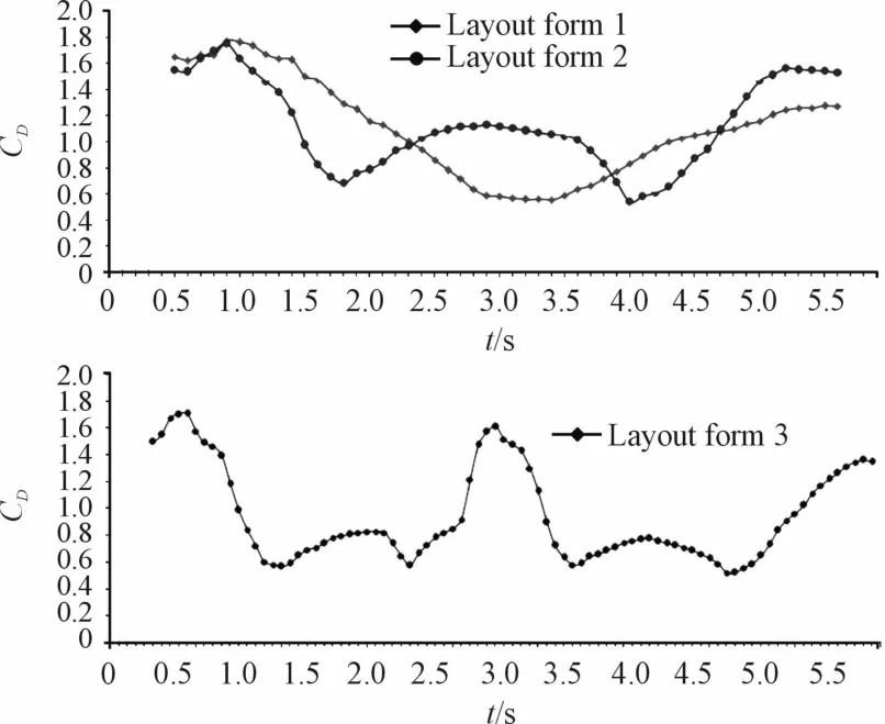
Fig.8 The variation curve of the d rag coefficient as the vehic Ie m oves for three Iayouts
4.1.2 Analysis of lateral force coefficient and lateral force
Fig.9 shows the variation of lateral force coefficient with time under three different building layouts.The overall trend ofCScurves in the first two layouts is the same.The lateral force coefficient for the first layout decreases from 4.0 at about 1 s to about 2.3 s,and then basically stabilizes at about 1.0.After 3 s,it slowly rises and eventually returns to its original level.Due to the slow decrease and increase,its influence on the driving stability and safety for heavy commercial vehicles is not as obvious as the second layout.For the second layout,the lateral force coefficient first slowly increases to about 5.5,and then rapidly decreases to below zero in less than 1s,that is,the direction of the lateral force changed.The lateral force coefficient decreases from about 1.7 s and the speed slows down and gradually stabilizes at about-1.5.After 3.5 s,theCSvalue begins to rise rapidly to nearly 4.0,and the direction of lateral force changes once more.Since then,the lateral force coefficient tends to stabilize and returns to the original levelwhen the body is far away from the building.For the second layout,the lateral force changes its direction twice in a short time,which is a dangerous thing.TheCScurve for the third layout can also be regarded as the superposition of the twoCScurves in the second layout.Affected by the mutual interference between the two buildings,the point at which the direction of lateral force changes is slightly changed and it changes four times during the driving.
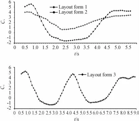
Fig.9 The variation curve of the IateraI force coefficient as the vehic Ie m oves for three Iayouts
Table 1 shows the lateral forces at 10 observation points aftert=0.8 s their rate of change relative to the values corresponding to the observation points att=0.8 s for the second layout.The lateral force reaches a peak value of 9.66 kN after 0.8 s of vehicle movement.After that,the lateral force has a dramatical change fromt=0.8 s tot=1.8 s.Themaximum variation of lateral force is up to-12 kN·s-1,that is,the lateral force decreases by 12 kN on average within 1 s,which may seriously affect the driving stability and safety under heavy crosswinds.
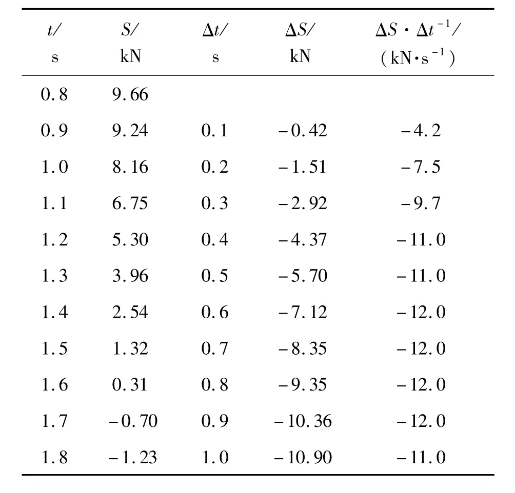
Tab Ie 1 Latera Ifo rce and change rates at ten observation poin ts after t=0.8 s for the second Iayou t
4.1.3 Analysis of Yawing Moment Coefficient and Yawing Moment
Fig.10 shows the variation law of yawing moment coefficient with time for three different building layouts.From the figure,it can be observed that the yawing moment coefficient changes significantly when the heavy commercial vehicle is approaching or away from the building.TheCYMvalue changes slowly and evenly for the first layout.Approximately,it decreases continuously in the firsthalf of the journey and increases gradually in the second half until it is up to the original level.For the second layout,the overall trend is also down first and then up,but the change is faster.In particular,fromt=3.9 s to 4.8 s,the yawing moment coefficient increases from-1.5 to about3.0.The distance between the observation pointatt=3.9 s and the pointt=3.2 s when the head of the vehicle starts to leave the boundary of the building is close to 1 time the vehicle length.This indicates that the position of the building boundary is notmuch related to the starting point at which the transient aerodynamic characteristics of heavy commercial vehicles changes under urban road conditions.Violent change of yawing moment coefficient can still be observed in the curve corresponding to the third layout.Furthermore,the rate of change is greater in the process ofmoving away from the building.In addition,CYMvalues for the second and third layouts both decrease slightly when the head of the vehicle begins to drive out of the boundary of the building,that is,the observation points att=3.2 s and 6.5 s.

Fig.10 The variation curve of the yaw ing mom ent coefficien t as the vehic Ie m oves fo r three Iayouts
Table 2 shows the yawingmoments at each observation point in the period oft=3.5-4.5 s for the third layout and the rate of change relative to the value at the observation point oft=3.5 s.The yawing moment for this layout reaches the lowest value of-9.47 kN·m at the observation pointwhent=3.5 s,and increases to 19.49 kN·m in less than one second,with themaximum rate of change 35 kN·m·s-1.In the case of heavy crosswind,the value will increase a lot,which will affect the driving safety for heavy commercial vehicles.
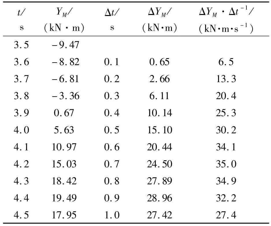
Tab Ie 2 Yaw ing m om ents and change rates at ten observation points after t=3.5 s for the third Iayout
4.2 Analysis of velocity in the flow field
In view of the law found by the analysis of variation of aerodynamic force,aerodynamicmoment and corresponding coefficient,the focus is put on the observation section in which the aerodynamic load of the vehicle body changesmore dramatically for each layout.
Fig.11-13 show the velocity distributions in the flow field around the building and the vehicle body at different observation points for the three layouts,respectively.For the convenience of comparison,the direction of crosswind for the first figure is from bottom to top.In the figure,the interaction between the vehicle body and the flow field around the building can be obviously observed during the movement.When heavy commercial vehicles are far away,the structure of the flow field around the building formed by the blocking effect of the building itself on the airflow is similar,and the low-speed zone is formed on its upwind side and downwind side.It can be seen from the three pictures that the low-speed zone in front or behind the building is wide enough to affect the flow field around heavy commercial vehicles.By comparing the structure of the downwind flow field of the building in Fig.12 and Fig.13,it can be found that although the flow field boundary at the gap for the third layout is squeezed and cannot fully develop,showing a linear state that is basically beam with the geometric boundary of the building,its effect on the transient aerodynamic characteristics of heavy commercial vehicles is similar to that of the second layout.
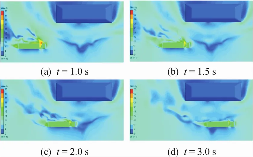
Fig.11 Ve Iocity contou r of the Z=1.5 m fo r the first buiIding Iayout

Fig.12 Ve Iocity contour of the Z=1.5 m for the second buiIding Iayout
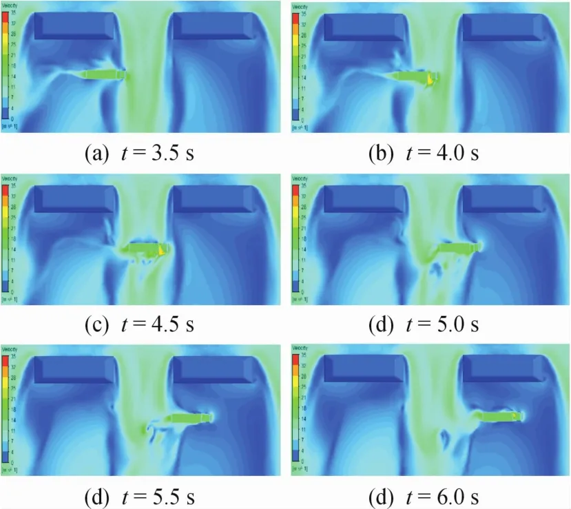
Fig.13 Ve Iocity contour of the Z=1.5 m for the third buiIding Iayout
After comprehensively comparing the velocity distribution cloud map for each layout and the variation laws of aerodynamic coefficient and resistance coefficient mentioned above,a conclusion can be drawn that the time point when the aerodynamic load begins to change dramatically is exactly the point when the vehicle body enters or exits the boundary of the building flow field.When the vehicle body completely enters the building flow field,the change amplitude weakens until it stopped.Therefore,the location of the flow field boundary formed by a building under the action of crosswinds rather than the geometric boundary of the building itself has a key influence on the transient aerodynamic characteristics of a heavy commercial vehicle.
5 Conclusions
The following conclusions can be drawn from this study:
(1)Urban buildings have a significant impact on the transient aerodynamic characteristics of heavy commercial vehicles.The influence of the buildings in the latter two layout schemes ismore prominent.The third scheme can be regarded as the superposition of the second along the time axis.
(2)For the second layout,the direction of lateral force changes from 9.66 kN to-1.23 kN withint=0.8-1.8 s,and the rate of change is close to-12kN·s-1.A similar phenomenon exists in the third scheme.The yawingmoment reaches theminimum of-9.47 kN·m and themaximum of 19.49 kN·m at the observation points oft=3.5 s andt=4.4 s,respectively.The rate of change reaches 35 kN·m·s-1within the same period.Moreover,in the process of vehiclemotion,the lateral forcewill change its direction,which has an impact on driving safety.
(3)According to the change law of aerodynamic load and the velocity distribution cloudmap,the time point when the aerodynamic load begins to change dramatically is exactly the time point when the vehicle body enters or exits the boundary of the building flow field.When the vehicle body completely enters the building flow field,the change amplitude weakens until it stops.
The actual conditions of urban road environment and surrounding buildings are diverse and complex.In the future research,the diversity of driving envi-ronment in the city should be enriched in order to better explore the aerodynamic laws of urban operating conditions.

- 机床与液压的其它文章
- Study on Face detection method based on lightweight convolutional neural network
- Application of genetic optim ization lvq neural network in equipment fault diagnosis system
- Research on sliding mode control of manipulator based on RBF neural network optim ized by bionic swarm intelligence
- Research on bearing fault diagnosis technology based on deep convolution neural network
- Research on the application of improved machine learning collaborative recommendation algorithm in intelligent control
- Design of liquid filling machine positioning system based on RBFneural network activedisturbance rejection controller