Influence of correlation scale errors on aquifer hydraulic conductivity inversion precision

Yun-xiao Mu ,Lei Zhu ,*,Tong-qing Shen ,Meng Zhang ,Yuan-yuan Zha

a School of Civil Engineering and Water Conservancy,Ningxia University,Yinchuan 750021,China

b Engineering Research Center for Efficient Utilization of Modern Agricultural Water Resources in Arid Regions,Ministry of Education,Yinchuan 750021,China

c State Key Laboratory of Water Resources and Hydropower Engineering Science,Wuhan University,Wuhan 430072,China

Received 11 July 2019;accepted 16 February 2020

Available online 28 September 2020

Abstract In order to investigate the influence of correlation scale error on the inversion precision of the hydraulic conductivity of the aquifer,the successive linear estimator(SLE)was used to invert the hydraulic conductivity field of a heterogeneous aquifer based on synthetic experiments.By increasing the numbers of observation wells and pumping tests,we analyzed the difference between the estimated and true values of hydraulic conductivity with different correlation scale errors.The relationships between the observation well number and the error in inversion results,and between the pumping test number and the error in inversion results were investigated.The results show that,if the amount of observed head data is insufficient,there will be errors in inversion results with changing correlation scale.Due to the existence of correlation scale error,the improvement of inversion precision gradually slows down with the increase of the amount of observed head data,which indicates that too much observed head data causes data redundancy.Therefore,for the synthetic experiments described in this paper,the observation well number should be less than 41,the pumping test number should be less than 17,and a more suitable method should be selected according to the precision requirements of specific situations in practical engineering.

© 2020 Hohai University.Production and hosting by Elsevier B.V.This is an open access article under the CC BY-NC-ND license(http://creativecommons.org/licenses/by-nc-nd/4.0/).

Keywords:Hydraulic conductivity;Parameter inversion;Successive linear estimator;Correlation scale error;Observation well number;Pumping test number

1.Introduction

Uncertain hydraulic parameters are crucial to groundwater flow modeling.The observed head data from pumping tests are usually used to invert these unknown parameters.However,the nonlinear relationship between head data and hydraulic parameters hinders the effectiveness of the inversion.Yeh's group presented an iterative cokriging technique,the successive linear estimator(SLE),which used a linear estimation method to introduce the nonlinear relationship between head and the hydraulic parameters of aquifers(Yeh et al.,1996;Zhang and Yeh,1997).SLE is a parameter-estimation method based on geostatistics.It has been successfully applied to parameter estimation of saturated and unsaturated zones(Yeh et al.,1995;Hanna and Yeh,1998;Hughson and Yeh,2000),hydraulic tomography(Zhu and Yeh,2005),and electrical resistivity tomography(Yeh et al.,2002;Hao et al.,2008).Many scholars have conducted research based on SLE(Bohling et al.,2002;Zhu and Yeh,2005;Cardiff and Barrash,2011;Jimenez et al.,2013;Jiang et al.,2017).In contrast to the kriging method,SLE considers the nonlinear relationship between head and the hydraulic parameters of aquifers,and reveals more detailed aquifer properties with the same amount of head data(Kitanidis and Vomvoris,1983;Hoeksema and Kitanidis,1984).Zhu and Yeh(2005)have developed a sequential successive linear estimator(SSLE),which reduces the computational cost by sequentially containing the information obtained from different pumping tests(Yeh and Liu,2000;Chen et al.,2014;Liu et al.,2002;Illman et al.,2007;Dong et al.,2009;Zha et al.,2015,2016).Xiang et al.(2009)have proposed a simultaneous successive linear estimator(SimSLE),which contains all the head data from different pumping tests,to estimate the hydraulic properties of aquifers.SimSLE provides more constraints for the inversion problem and presents a higher convergence speed than SSLE(Xiang et al.,2009).

For specific research areas,the properties of any point in space are definite.If we know the measured data of a point in space,then the spatial distribution of its properties is determined.However,due to the limitations of observation technology and measurement cost,it is impossible to obtain the hydrogeological parameters of every point in the soil(Tang et al.,2012).Through numerical experiments,Yeh and Liu(2000)concluded that when there were enough observed head data,the variance and correlation scale of the estimated values of hydraulic parameters used for inversion had little influence on inversion results(Zhao et al.,2015).However,in practice,the number of observation wells is much less than the number of nodes required in numerical models,and the prior understanding of the correlation scale contains errors.This study aimed to investigate the influence of correlation scale error on inversion precision with different amounts of observation data based on synthetic experiments.

2.Model description

2.1.Successive linear estimator

SLE was developed with the kriging and cokriging methods(Yeh et al.,1995;Hughson and Yeh,2000;Zhang and Yeh,1997).SLE calculates the head h field using the groundwater flow governing equation,and the corresponding hydraulic conductivity K field is obtained from the kriging or cokriging method to determine the difference between the observed and estimated values at each observation point.These differences are applied to the linear estimation to modify the initial estimated value of K,which is subsequently used to calculate the new head field.The differences between the observed head value and the modified head value at each observation point are obtained again.Then,the differences are replaced by the linear estimation to further modify the estimated value of K.This process iterates until the misfit error is stable or can be ignored(Yeh et al.,1996;Ye,2017).Considering the case in which head during a steady-state flow condition is used to estimate the hydraulic conductivity,SLE takes the following form:

where xmand xjrepresent observation points;^f（k）（xm）is the previous estimate at xmmade using the kriging or cokriging method;h*（xj）and h（k）（xj）are the observed and simulated head values,respectively,at observation location xj;the superscript k is the iteration index;represents the contribution of the difference between the observed value and the estimated value of h at xjto the estimated value of f at xmat the kth iteration;and n represents the total number of observation points(Zhang and Yeh,1997;Xiang et al.,2009;Ye,2017).

2.2.Evaluation criteria for inversion results

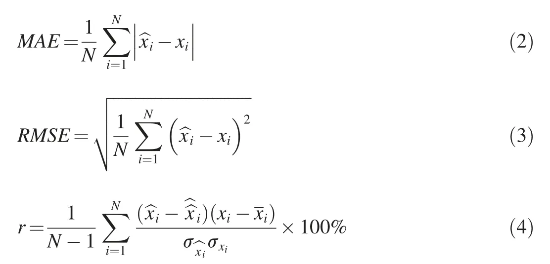
The mean absolute error MAE,root mean square error RMSE,correlation coefficient r,and determination coefficient R2are used as the criteria to evaluate the error of SLE inversion results.The mathematical expressions of MAE,RMSE,and r are as follows:

3.Numerical experiments

The numerical experiments were based on variably saturated flow and transport utilizing the modified method of characteristics,in two dimensions(VSAFT2),a model developed by Yeh et al.(1993).VSAFT2 can execute forward calculation and groundwater parameter inversion of twodimensional groundwater flow.Its core algorithm is SLE,and the simulation results can be displayed and postprocessed with Tecplot 360.

3.1.Synthetic experiments

The study area is a horizontal two-dimensional heterogeneous aquifer of 10 km×10 km.The mean value of the hydraulic conductivity K is 6.5 m/d;the variance of lnK is 4;the correlation scale of K values in the x and y directions is 3.0 km;the upper boundary and lower boundary are constant head boundaries,with values of 5 m and 4 m,respectively;and the left and right boundaries are impermeable boundaries.In the experiment,a pumping well P1 with a flow rate of 3 000 m3/d was set.The material field of hydraulic conductivity K is shown in Fig.1,and the head results of the synthetic experimental study area are shown in Fig.2,in which the white dots represent observation wells,and the red dot represents the pumping well.

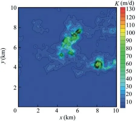
Fig.1.Material field of hydraulic conductivity.

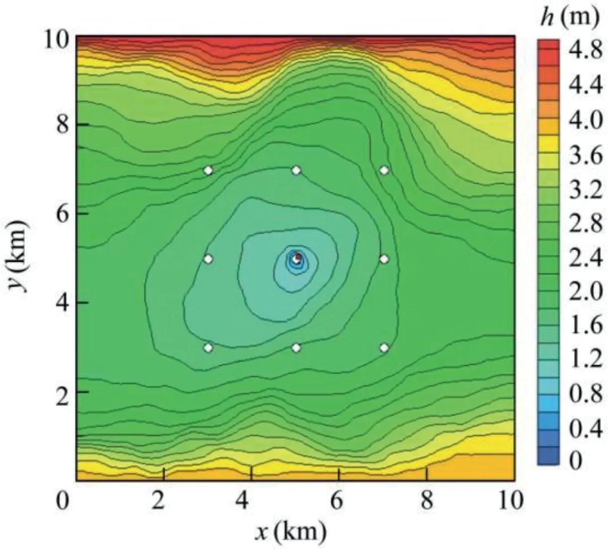
Fig.2.Contour map of head.

3.2.SLE parameter inversion

The setting of the study area,the hydraulic conductivity,and the boundary conditions of SLE parameter inversion were the same as the settings of the synthetic experiments.The correlation scale of K was the same in the x and y directions,and was changed based on the synthetic experiments.The head values calculated from the synthetic experiments were used as observed values in parameter inversion to obtain the spatial distribution of the hydraulic parameter estimation values.In scenario 1,with the change of the correlation scale,the observation well number(nw)was increased in turn(from 9 to 25,41,57,73,and 81)for parameter inversion.In scenario 2,the pumping test number(nt)was increased in turn(from 1 to 17,33,49,and 65)for parameter inversion.The values and errors of the correlation scale are shown in Table 1.

Table 1 Values and errors of correlation scale.

4.Results and discussion

4.1.Inversion results of synthetic experiments

4.1.1.Increased observation well number

The parameter inversion results when the correlation scale in parameter inversion is 3.0 km(which is the same as that in the true field in synthetic experiments)and the observation well number is nine are shown in Fig.3.

The parameter inversion results using the correlation scale of 1.5 km as an example,with the observation well number increasing from 9 to 81 are shown in Fig.4 and Fig.5.

When the estimated value of lnK deviates more from the true value,the error between the estimated value and true value is larger.Through comparison,it can be seen from Fig.3(b)and Fig.5(a)that the estimated lnK obtained through inversion is more scattered and more deviated from the true value when the correlation scale is 1.5 km,as compared with that when the correlation scale is 3.0 km,indicating that the error in inversion results increases when the correlation scale is decreased.

Fig.5 shows that for the correlation scale of 1.5 km,when only nine observation wells are used to invert hydraulic conductivity,the inversed hydraulic conductivity field is relatively dispersed and the deviation of the inversion results from the true value is large.When the observation well number increases from 9 to 25,41,57,73,and 81,the inversed hydraulic conductivity moves closer and closer to the true value,with R2increasing from 0.07 to 0.39,0.51,0.54,0.57,and 0.58,respectively.Therefore,with the increase of the observation well number,there is a gradual decrease in the error of the estimated hydraulic conductivity value and an improvement of the inversion precision.

4.1.2.Increased pumping test number

Using the correlation scale of 1.5 km as an example,when the observation well number is nine,and the pumping test number is increased from 1 to 65,the parameter inversion results are shown in Figs.6 and 7.

Fig.7(a)shows that for the correlation scale of 1.5 km,when the pumping test number is only one,the inversed hydraulic conductivity field is relatively dispersed,and the deviation of the inversion results from the true value is large.When the pumping test number is increased from 1 to 17,33,49,and 65,the estimated values of hydraulic conductivity gradually approach the true value,with the R2value increasing from 0.07 to 0.81,0.87,0.90,and 0.91,respectively,showing that with the increase of the pumping test number,the error of the estimated values of hydraulic conductivity gradually decreases,and the inversion precision is improved.

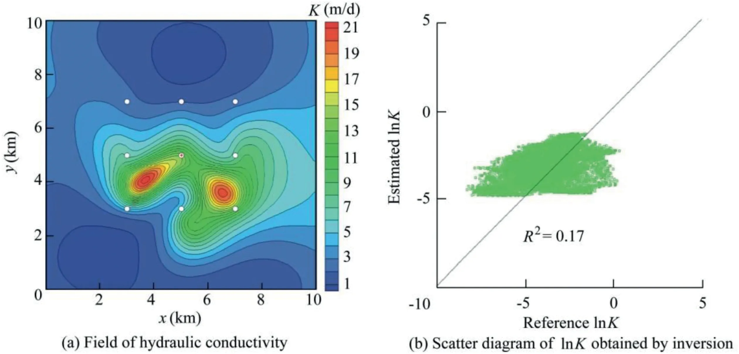
Fig.3.Inversion results of hydraulic conductivity at a correlation scale of 3.0 km.

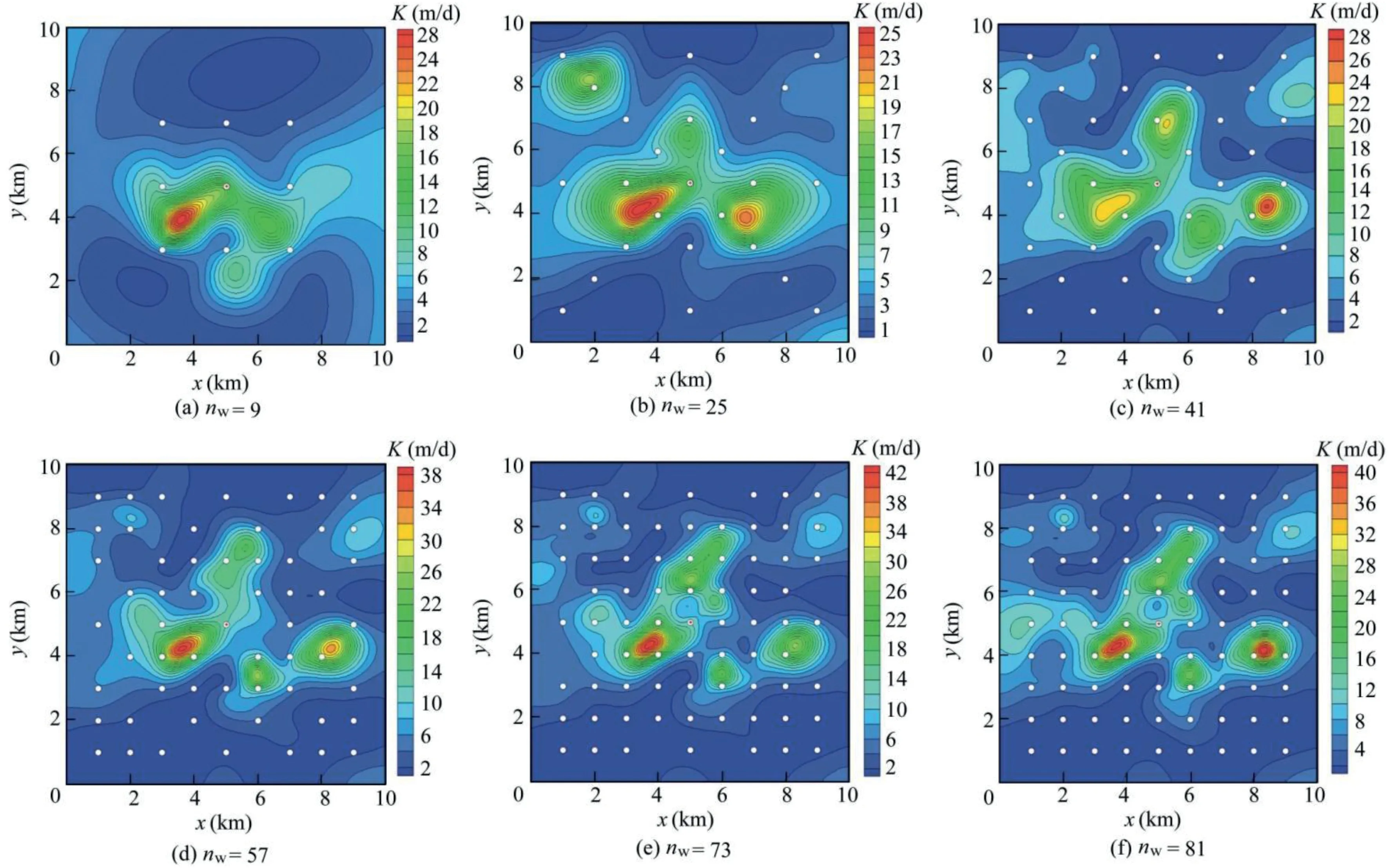
Fig.4.Field of hydraulic conductivity at a correlation scale of 1.5 km with increasing observation well number.

4.2.Error analysis

4.2.1.Increased observation well number

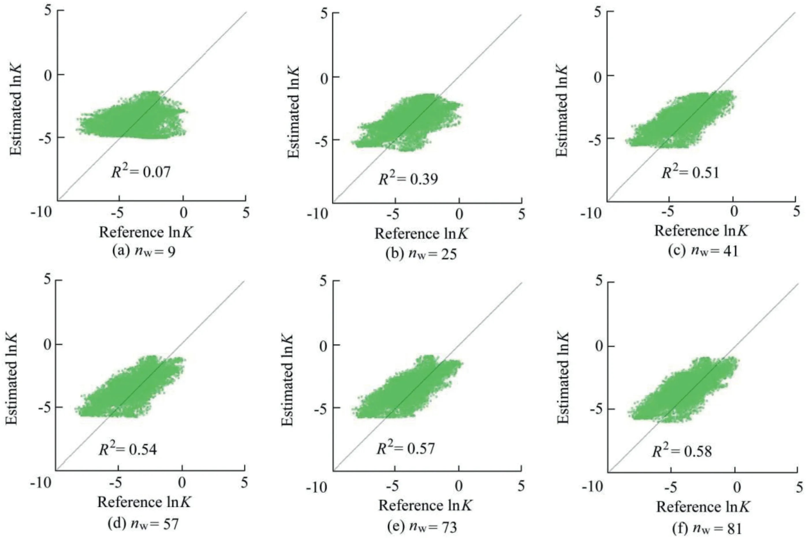
Fig.5.Scatter diagram of lnK at a correlation scale of 1.5 km with increasing observation well number.

Fig.6.Field of hydraulic conductivity at a correlation scale of 1.5 km with increasing pumping test number.

The variations of the inversion result error with different observation well numbers and inversion correlation scale values when the pumping test number is one are shown in Fig.8.When the correlation scale is decreased by 10%-90%,the inversion result errors MAE and RMSE decrease when the observation well number is less than 41,while r and R2increase.When the observation well number is greater than 41,changes in MAE,RMSE,r,and R2diminish.Table 2 shows the variations of R2with the observation well number for the correlation scale errors of－50%and－90%.The results show that the precision is improved more rapidly when the observation well number is less than 41,compared with when the observation well number is greater than 41.

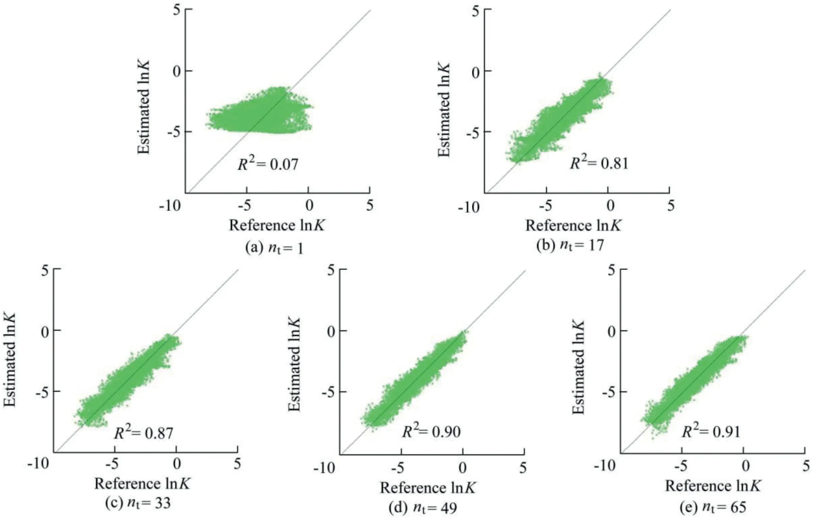
Fig.7.Scatter diagram of lnK at a correlation scale of 1.5 km with increasing pumping test number.

The variations of the inversion result error with the increas e of inversion correlation scale value at different numbers of observation wells are shown in Fig.9.When the correlation scale is increased by 10%-100%,MAE and RMSE decrease,and r and R2increase when the observation well number is less than 41.When the observation well number is greater than 41,MAE,RMSE,r,and R2flatten and the changes become relatively small.Table 3 shows the variations of R2with the observation well number for the correlation scale errors of 50% and 100%.The results show that the precision is improved more rapidly when the observation well number is less than 41,compared with when the observation well number is greater than 41.

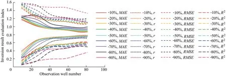
Fig.8.Relationship between observation well number and inversion result evaluation indices of MAE,r,RMSE,and R2 with reducing correlation scale.

4.2.2.Increased pumping test number

The variations of the inversion result error with the decrease of inversion correlation scale value at different pumping test numbers when the observation well number is nine are shown in Fig.10.When the correlation scale is decreased by 10%-90%,the values of MAE and RMSE decrease with a pumping test number less than 17,and the r and R2values increases.When the pumping test number is greater than 17,changes in MAE,RMSE,r,and R2diminish.It should be noted that when the correlation scale error is－90%,increasing the pumping test number cannot reduce the inversion result error since the correlation scale error is too large.Table 4 shows the variations of R2with the pumping test number for the correlation scale errors of－50% and－90%.The results show that the precision is improved more rapidly when the pumping test number is less than 17,compared with when the pumping test number is greater than 17.

Table 2 Variation of R2 with observation well number for correlation scale errors of－50% and－90%.

Fig.9.Relationship between observation well number and inversion result evaluation indices of MAE,r,RMSE,and R2 with increasing correlation scale.

Table 3 Variation of R2 with observation well number for correlation scale errors of 50% and 100%.

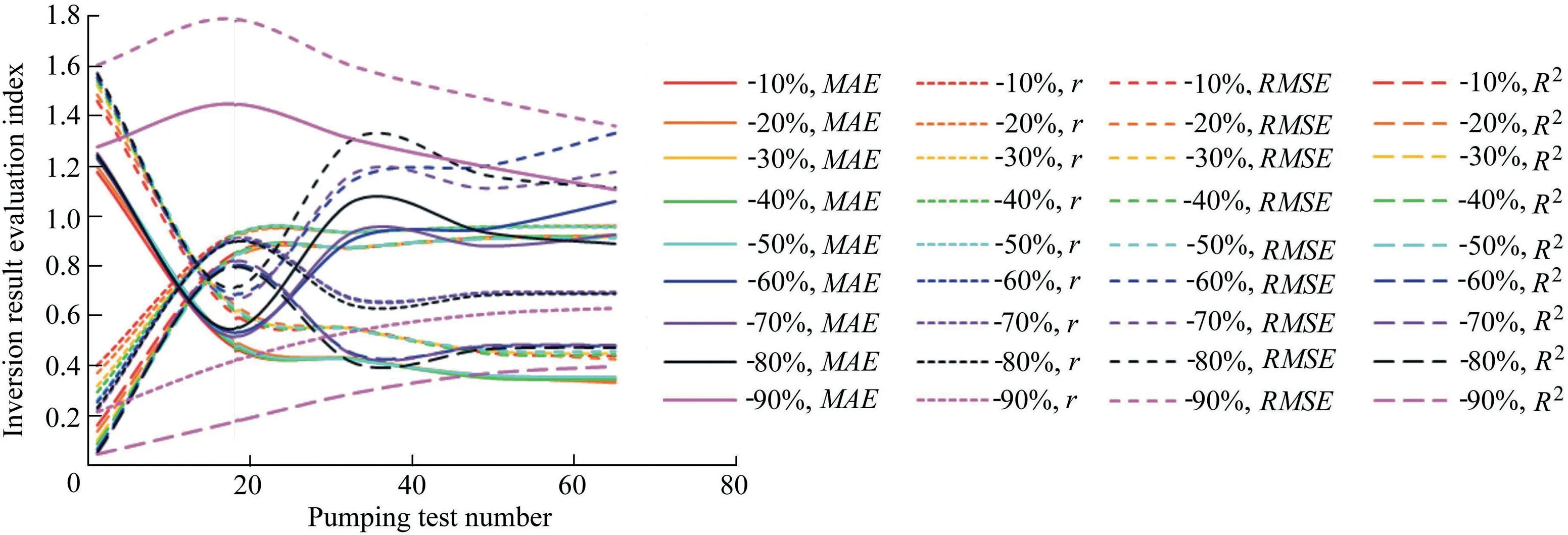
Fig.10.Relationship between pumping test number and inversion result evaluation indices of MAE,r,RMSE,and R2 with reducing correlation scale.

Table 4 Variation of R2 with pumping test number for correlation scale errors of－50% and－90%.

Based on the correlation scale of 3.0 km in synthetic experiments,with the increase of inversion correlation scale value,the variation of inversion result error with different pumping test numbers is shown in Fig.11.When the correlation scale is increased by 10%-100% and the pumping test number is less than 17,MAE and RMSE decrease,while r and R2increase.When the pumping test number is greater than 17,MAE,RMSE,r,and R2begin to flatten gradually and the change becomes relatively small.Table 5 shows the variations of R2with the pumping test number for the correlation scale errors of 50%and 100%.The results show that the precision is improved more rapidly when the pumping test number is less than 17,compared with when the pumping test number is greater than 17.

Fig.11.Relationship between pumping test number and inversion result evaluation indices of MAE,r,RMSE,and R2 with increasing correlation scale.

Table 5Variation of R2 with pumping test number for correlation scale errors of 50% and 100%.

5.Discussion

It can be seen from Figs.8 and 9 that,when there are nine observation wells,the inversion result errors are large due to the small amount of observed head data and the existence of correlation scale errors.As shown in Figs.10 and 11,when there is only one pumping test,the inversion result errors are large due to the small amount of observed head data and the existence of correlation scale errors.With the increase of observation well number and pumping test number,the errors in inversion results diminish,and the inversion precision is improved gradually,but the rate of improvement slows.For example,when the correlation scale is 2.7 km(relative error of－10%)and the observation well number increases from 9 to 41(increases by 39.5%),the inversion precision is improved by 237%;when the observation well number increases from 41 to 81(increases by 49.4%),the inversion precision is only improved by 15%.When the pumping test number increases from 1 to 33(increases by 40.7%),the inversion precision is improved by 443%;when the pumping test number increases from 33 to 65(increases by 39.5%),the inversion precision is only improved by 5.7%.The reason is as follows:the error in the inversion result is caused by the correlation scale error,the insufficient observed head data amount,and the numerical calculation error.The errors in the inversion result caused by the correlation scale error and the insufficient observed head data amount are offset gradually with the increase of observation well number and pumping test number.However,the numerical calculation error cannot be eliminated,which will become more apparent with a large number of observation wells and pumping tests.

In terms of improving inversion precision,based on the correlation scale of 3.0 km in synthetic experiments,the inversion correlation scale value is changed.For a correlation scale error of－50%,the determination coefficient is 0.51 when the observation well number is 81;while the determination coefficient increases to 0.84 when the pumping test number is 65.For a correlation scale error of 50%,the determination coefficient is 0.37 when the observation well number is 81;while the determination coefficient increases to 0.67 when the pumping test number is 65.Considering that the method of increasing the pumping test number needs less wells than the method of increasing the observation well number,for a constant correlation scale error,increasing the pumping test number is more effective than increasing the observation well number.However,when the observation well number is greater than 41 and the pumping test number is more than 17,the variations of MAE,RMSE,r,and R2begin to flatten gradually and the change becomes relatively small.Therefore,for the synthetic experiments described in this paper,in order to obtain better inversion results,we can select the observation well number less than 41 and the pumping test number less than 17 to inverse the hydraulic conductivity of aquifers.However,when the error of the correlation scale is too great,it is difficult to obtain the ideal inversion result no matter which method is used.

6.Conclusions

(1)When the amount of observed head data is insufficient,changing the correlation scale based on the value in synthetic experiments will introduce errors into the inversion results of hydraulic conductivity.

(2)With the correlation scale error,the inversion precision of aquifer hydraulic conductivity increases rapidly with the observation well number and the pumping test number at first,then the improvement of inversion precision slows down when the observation well number and the pumping test number are increased to certain numbers.This is mainly due to the fact that with the increase of observed head data amount,the errors caused by correlation scale error and the insufficient observed head data amount are gradually offset,while the errors of numerical calculation become more and more apparent.For the synthetic experiments in this paper,the observation well number should be less than 41,and the pumping test number should be less than 17.

(3)When the precision of inversion results is required to be high,it is recommended to adopt the method of increasing the pumping test number.When the inversion precision is not required to be particularly high,it should be considered to increase the observation well number,because this method has the advantages of higher computational efficiency and less time than the method of increasing the pumping test number.If the correlation scale error is too great,no matter which method is used,it is difficult to obtain the ideal inversion results.Determination of which method is better should still include consideration of the economic benefits,which is not discussed in this paper.

(4)The results reveal that the correlation scale is crucial for inversion results if the amount of observed head data is insufficient,which should be measured before the synthetic experiments.The correlation scale can be obtained by measuring the saturated hydraulic conductivity of a geologic medium at some intervals along a transect line.It is assumed that this geologic medium consists of many clay lenses.Intuitively,we would expect that pairs of hydraulic conductivity values measured at intervals within a clay lens will be highly correlated,and measurements taken at intervals greater than the dimension of the clay lens are uncorrelated.

Declaration of competing interest

The authors declare no conflicts of interest.