Simulation of Silty Clay Compressibility Parameters Based on Improved BP Neural Network Using Bayesian Regularization1

CAI Run ,PENG Tao ,WANG Qian ,HE Fanmin and ZHAO Duoying

1)Chengdu Surveying Geotechnical Research Institute,Co Ltd.of MCC,Chengdu 610023,China

2)Key Laboratory of Loess Earthquake Engineering,Gansu Earthquake Agency,Lanzhou 730000,China

3)Lanzhou Institute of Seismology,China Earthquake Administration,Lanzhou 730000,China

Soil compressibility parameters are important indicators in the geotechnical field and are affected by various factors such as natural conditions and human interference.When the sample size is too large,conventional methods require massive human and financial resources.In order to reasonably simulate the compressibility parameters of the sample,this paper firstly adopts the correlation analysis to select seven influencing factors.Each of the factors has a high correlation with compressibility parameters.Meanwhile,the proportion of the weights of the seven factors in the Bayesian neural network is analyzed based on Garson theory.Secondly,an output model of the compressibility parameters of BR-BP silty clay is established based on Bayesian regularized BP neural network.Finally,the model is used to simulate the measured compressibility parameters.The output results are compared with the measured values and the output results of the traditional LM-BP neural network.The results show that the model is more stable and has stronger nonlinear fitting ability.The output of the model is basically consistent with the actual value.Compared with the traditional LMBP neural network model,its data sensitivity is enhanced,and the accuracy of the output result is significantly improved,the average value of the relative error of the compression coefficient is reduced from 15.54%to 6.15%,and the average value of the relative error of the compression modulus is reduced from 6.07%to 4.62%.The results provide a new technical method for obtaining the compressibility parameters of silty clay in this area,showing good theoretical significance and practical value.

Key words:Silty clay;Compressibility;Correlation analysis;Bayesian regularization;Neural networks

INTRODUCTION

Soil compressibility is an important parameter in the field of geotechnical research.Due to the fact that soil particles are incompressible,the change of soil volume is thus equal to the change of the entire pore volume.Besides,soil compressibilty is not a constant and is associated with the stress variation.A majority of previous studies focus on changing several influencing factors to obtain the corresponding compressibility parameters of silty clay.Limited to the difference in test conditions and test methods,the conclusions are also various.As a result,there is currently no well-acknowledged model for silty clay compressibility parameters that fits perfect with the actual condition.Because of the strong ability of non-linear fitting and approximation,artificial neural network can make up for the defects of traditionally empirical model,attracting more attention from domestic and foreign scholars (Wang Jiaxin et al.,2018;Goh A.T.C.,1995;Orbanic P.et al.,2003;Hinton G.et al.,2012;Hinton G.E.,2007;Smith S.M.et al.,2015;Cai Run et al.,2018).With new insights for modeling the unknown nonlinear systems,neural network has been successfully applied in the field of geotechnical engineering.(Wang Caijin et al.,2019;Wang Maohua et al.,2019;Huang Faming et al.,2018;Gao Jie et al.,2018;Liu Houxiang et al.,2018).In detail,using ANFID neural network,Zhu Shimin et al.,(2019) propose a creep model for red clay with the consideration of confining pressure and deflection stress.Also,a BP network model for strength prediction of steel slag is established by Li Xinmin(Li Xinmin et al.,2017).Based on the field-measured data and parameter sensitivity analysis,the key parameters of stratum are determined,and the dynamic construction inversion analysis method based on parameter sensitivity analysis and BP neural network is proposed by Xiao Mingqing (Xiao Mingqing et al.,2017).In the neural network model,generalization ability is the most important index to measure the network performance,and the network without generalization ability has no practical significance.The generalization ability of neural network is related to the training sample and network structure.The limitations of the traditional BP neural network (i.e.,learning algorithm is LM-BP) has the following disadvantages (Cai Run,2018):(1) It is highly sensitive to the initial weights;(2) the learning and memory of the network is unstable;(3) the BP algorithm easily makes the weights fall into local minima;(4) the learning of traditional neural networks is prone to over fitting.Moody claims that the main reason for over fitting is the redundancy of network structure (Moody J.E.,1992).Therefore,some scholars indicate some improved methods.Taking the advantage of genetic algorithm for weight optimization,Rao Yunkang et al.,(2019) establish a prediction model for maximum dryness density,providing a reference for compaction quality control as well as gravel soil selection that both meet the requirements of engineering compaction performance.Furthermore,by optimizing the relevant parameters of the output layer and hidden layer of the neural network,the model built by this method can effectively reduce the time cost and improve the accuracy of geological disaster monitoring and early warning (Wang Fang et al.,2019).Wang Shudong et al.,(2019) combine the Artificial Fish School Algorithm (AFSA) and the Elman network and then apply them to the slope stability judgement,obtaining expected results that have higher accuracy,better convergence,and more suitable slope displacement prediction.When the traditional BP neural network is used to calculate the compressibility parameters of silty clay,the output results are discrete.With the robust theoretical basis,Bayesian regularization makes full use of the relationship between input and output.This method introduces a priori distribution in the model parameters and optimize the solutions by constraining the output function.Importantly,it can prevent over-fitting by modifying the loss function.It also solves the problem of high calculation and local extreme values,stabilizing the output model and thus determining the soil compressibility parameters more accurately.

This paper builds an output model based on correlation analysis (SPSS) and Bayesian regularization algorithm to improve the BP neural network (BR-BP).Firstly,the main factors that affect the compressibility of the sample are checked by correlation analysis,for the purpose of avoiding the lengthy input information caused by subjective factors,thereby reducing the calculation dimension and improving the convergence performance of the network.Secondly,by optimizing the parameters of Bayesian regularization BP neural network,the defect that its calculation result is easy to fall into the local minimum value is effectively solved,thereby improving the output accuracy.Finally,the paper compares the established output model and the traditional LM-BP neural network output model through the test data of a project in Jianyang City.The results show that our improved model can significantly improve the output accuracy and can be used as a powder in the region.To conclude,it can be used as a feasible technical process and method for the output of clay compressibility parameters.

1 METHOD

1.1 One-dimensional Compressibility Index

The deformation characteristics of soil are very complicated,not only closely related to the basic properties of the soil,such as composition,state,and structure,but also related to the stress conditions (stress level,deformation conditions) of the soil.The compressibility of soil refers to the characteristic that the volume of soil shrinks under the action of vertical pressure when the pressure is equal in all directions or the lateral limit.At present,the most commonly used indoor test for determining the soil compressibility parameters is the lateral compression test,also known as the consolidation test.The commonly used compression indicators are the compression coefficientaand the compression modulusEs.The limits of the indicators are shown in Table 1:

Table 1 Limits of compressibility parameters

1.2 Neural Network Principle

The Back Propagation neural network,which is proposed by Rumelhart and McClelland in 1986,is a multi-layer forward neural network (Peng Lishun et al.,2019).The neural network model of BP algorithm has reached 80%-90% according to Cai Run et al.,(2018).The learning process of BP neural network mainly includes two processes:forward propagation of information and error back propagation.Fig.1 shows a three-layer BP neural network,including the input layer,hidden layer and output layer.Each neuron in the input layer is responsible for receiving the input information and passing it to each neuron in the middle layer;The hidden layer is the internal information processing layer,which is responsible for information transformation.At present,the most common method for determining the number of nodesJin the hidden layer is the trial and error method;the output layer is responsible for outputting the information of each neuron.The forward process includes the input information passing through the hidden layer to the output layer from the input layer and completing a forward learning process through the operation of the function.If the actual output does not match the expected output,the back-propagation phase of the error is entered.The error signal is returned along the original input route.Meanwhile,the error passes through the output layer,updating the weights and biases of each layer through error gradient descent algorithm.Such process continues until the sum of the error squares and the expected value reach the size of the set error value or the preset learning times.Forward and reverse processes are used repeatedly to determine the final output value size.

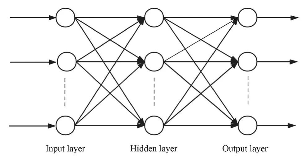
Figure 1 The BP neural network structure

The training performance function of artificial neural network adopts loss function(mean square error function)Ee,which is defined as:

In formula(1):nis the number of samples,kis the number of neural network output,ykis the expected output value,andAkis the actual output.

1.3 Bayesian Regularization Method

The Bayesian neural network method combines Bayesian method with neural network method.This paper introduces the Bayesian principle into the weight and the threshold of the neural network.The posterior probability of the weight is used as the optimization objective function,and the weight of the neural network is obtained by maximizing the posterior probability of the weight,solving the problem that the BP algorithm easily leads to the weight to fall into the local minimum value.For ordinary neural networks,the loss function needs to be designed,and the optimal parameters can be optimized by SGD,Adam and other optimizers to minimize the error.However,for Bayesian neural networks,it is the KL divergence that needs to be minimized.The regularization theory modifies the loss function for the purpose of preventing the occurrence of overfitting,improving the generalization ability of the network.Overfitting may occur if regularization terms are not added into the formula (Mackay D.J.C.,1992;Wong M.L.et al.,2004).In this paper,we adds a penalty termEwto the Bayesian regularization optimization algorithm to achieve a suitable fit,and then alleviates the problem of slow convergence and low learning efficiency of traditional neural network algorithms.The network performance function is as follows:

In the formula:Ewis the square sum of all network weights;EDis the error value between the output value and true value of each layer;aandbare regularization coefficients of performance function,also called hyper-parameters which control the distribution of weights and thresholds of the neural network,thus affecting the training effect.Whena≤b,as the number of training increases,the error of training samples becomes smaller,resulting in the network overfit phenomenon;Whena≥b,as the number of training increases,the weights become smaller,smoothing the network output.It will also produce the phenomenon of underfitting.

Under the Bayesian theory,we can obtain the formula as follows:

In the formula:γis the effective weight number,which represents the number of connection weights of the neural network that can reduce the training error,nis the total number of neural network parameters,γ==n -aTrace(H)-1;His the Heather matrix of the performance function,H=a▽2Ew+b▽2ED.It can be approximated by Gauss-Newton iteration method,λiis theith eigenvalue of matrixH.The flow chart of the Bayesian neural network algorithm program designed by the thesis is shown in Fig.2:

Figure 2 Flow chart of the structure and process

2 MODEL BUILDING AND EMPIRICAL ANALYSIS

2.1 Sampling Area

The sampling location,Longya Village,is situated in the south of Jianyang City,Sichuan Province.This area belongs to eroded shallow hill landform,most of which are agricultural.The micro-geomorphic units are shallow hillside landform and shallow hill valley landform (Fig.3).According to the results of drilling,in-situ testing and indoor geotechnical tests,the strata in the site are mainly Quaternary artificial accumulation layersand Quaternary slope alluvial layers().The sampling depth of silty clay is 0.4 m-18.3 m,the measured compression coefficient is 0.22-0.56,and the compression modulus is 3.27-7.75.Among them,40 sets of samples are used as test objects,20 sets of samples are used as training samples of the Bayesian regularization neural network,10 sets of samples are used as verification samples of the Bayesian regularization neural network,and the remaining 10 sets of samples are used as test data.

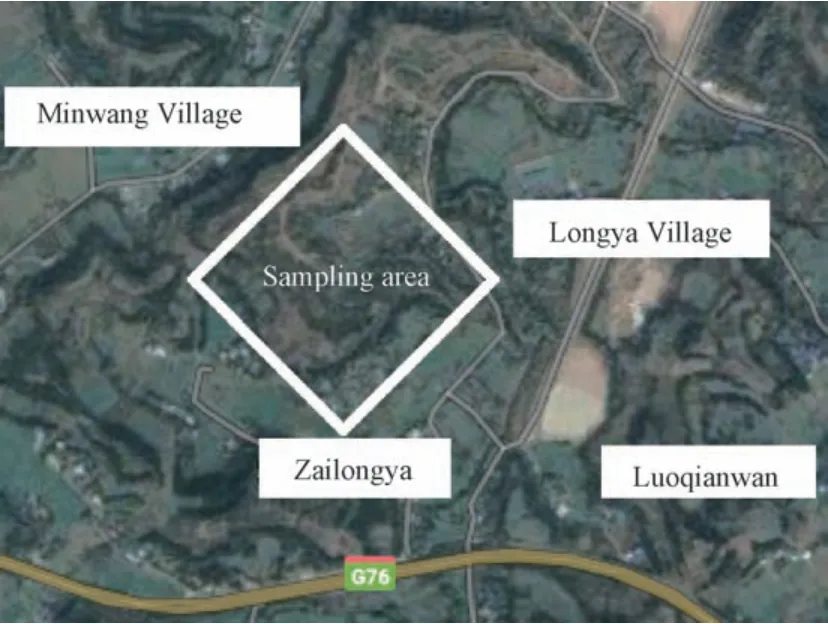
Figure 3 Site geomorphology and scope

2.2 Data Processing

Since there are numerous factors affecting the compressibility index of silty clay,and the coupling relationship between the compressibility index and the test conditions is complex,this paper selects the physical property parameters of the soil as the input of the model,and analyzes the correlation between the physical property parameters and the compressibility parameters to obtain the correlation coefficient (Pearson) of each parameter with the compressibility parameters,the results are shown in Table 2.

Table 2 Correlation of factors affecting compression parameters

From the table above,we can see that the correlation between each influencing factor and compressibility is different.According to the actual situation,we choose highly correlated and moderately correlated indicators,respectively (the absolute value of the correlation coefficient is greater than 0.5).No consideration will be given to low-level related factors.Finally,the most relevant indexes such as densityρ(g/cm3),water contentω(%),porositye,porosityn(%),and liquidity indexILare selected as the input of the model.

The great change in all collected data is not conducive to the training of neural networks.In order to avoid neuron saturation during training,the sample data is normalized and the output results are denormalized.The larger input values should still fall when the transfer function gradient is large.There are two purposes of doing this.Firstly,it is easy to facilitate data processing;Secondly,it can speed up the convergence of the program when it runs (Peng Lishun etal.,2019).Assuming that the dataX=(Xi) is normalized toX′=(X′i),the calculation formula of the normalization process is as follows:

Among them:YmaxandYminare artificially specified upper and lower bounds,in this paper,we setYmax=1 andYmin=0.

XmaxandXmincorrespond to the maximum and minimum values in the sample data,and satisfies the requirement Xmin≤X′≤Xmax.

Normalized and anti-normalized handler code in MATLAB are:

The training sample data are shown in Table 3:

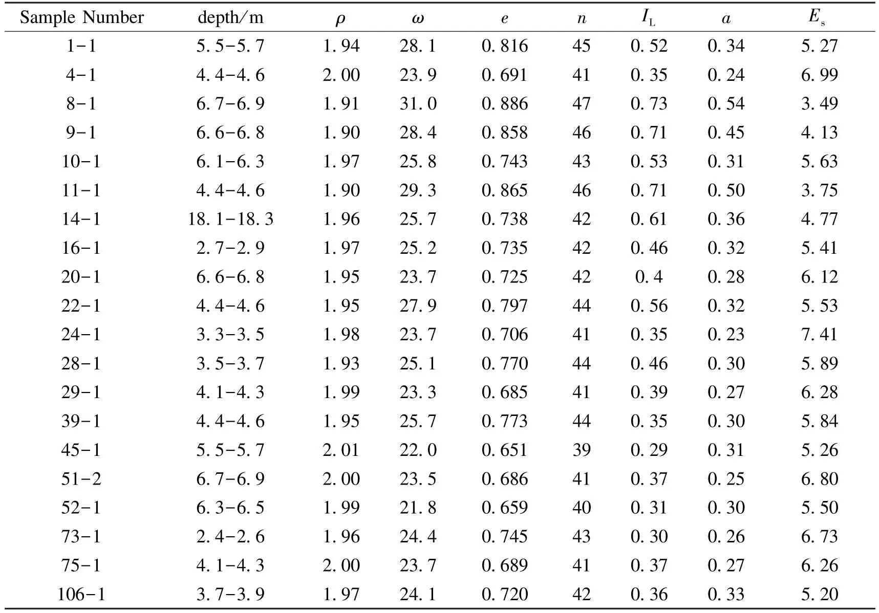
Table 3 Training samples

The neural network model has five input neurons.The tansig function is selected from the input layer to the hidden layer,and the purelin function is selected from the hidden layer to the output layer.Comparing the convergence curves of the two training functions(Fig.4):When the error performance of the BR-BP neural network model is reduced to the target value,the training is stopped.However,because the training speed of the LM-BP neural network model is too fast,each time the training is stopped,the network error performance drops far below the target value,which is prone to overfitting.This is also the reason why LM-BP neural network has poor promotion ability compared to BR-BP neural network.

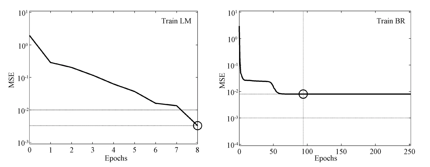
Figure 4 Convergence curves

This paper selects a hidden layer node numberJaccording to the empirical formulaJ=2 ×n +1,in whichnis the number of input units.By continuously changing the number of hidden layer neurons,we observe the test error value until the neural network converges.This paper also uses a trial and error method to determine the number of hidden layer nodes,testedJ=10,11,12,13,14,15 are finalized the number of hidden layer nodes is 14.

In order to maintain the efficient training capabilities of the neural network,we set the related parameters reasonably.The other parameter settings of the neural network model are shown in Table 4.The data samples are trained according to the network structure set by the parameters,and the training stops when the target accuracy is reached.

Table 4 Setting of training parameters for bayesian neural network

The method to calculate the influence degree of each input variable on the weight of the output variable uses the weights proposed by Garson.It calculates the weights of compression coefficient and compression modulu respectively(Garson G.D.,1991).The calculation formula is as follows:

In formula(6):Ihis the influence weight of thehinput parameter on thenoutput variable;NiandNjare the number of nodes in the input layer and hidden layer;ωijis the weight of the input layer to the hidden layer;νjtis the weight of the hidden layer to the output layer;The subscriptsh,mandnrepresent the corresponding neurons in the neural network model.The larger the value ofIh,the greater the proportion of its influence weight,and the greater its impact on the output.

After calculation,the final weights and thresholds of the neural network model based on BR-BP are obtained in Table 5 and Table 6.The weight of the input variable to the hidden layer and the hidden layer to the output variable indicate the relative magnitude of the influence of the input variable on the output variable.

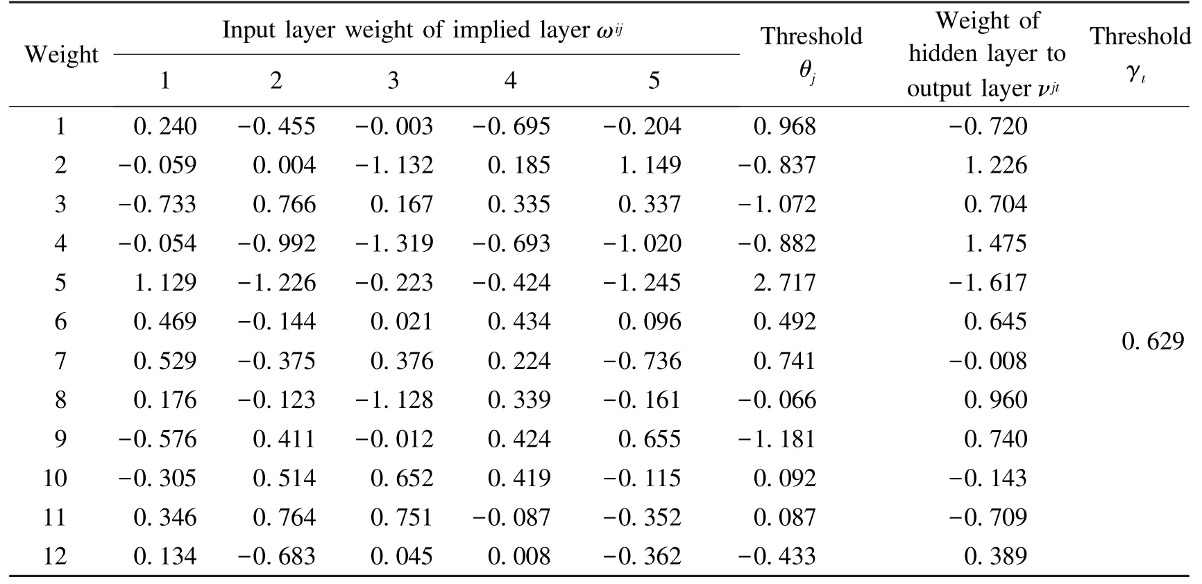
Table 5 Weights and thresholds(compression coefficient)

Garson weight coefficient calculated by formula(6)is shown in Fig.5.Among the five selected influencing factors,the influence degree on the compression coefficient is relatively uniform,among which the water content and liquidity index are relatively prominent.However,among the influence degree from the five factors on the compression modulus,the proportion of porosity and water content is larger,and the proportion of density is smaller.This shows that in this model the density has the smallest effect on the output of the compression modulus,and the porosity and water content have a greater effect.

Using the established BR-BP neural network model and the traditional LM-BP neural network model,the verification data (Table.7) are used to verify the compression coefficient and compression modulus respectively.The fitting results are shown in Fig.6 and Fig.7:

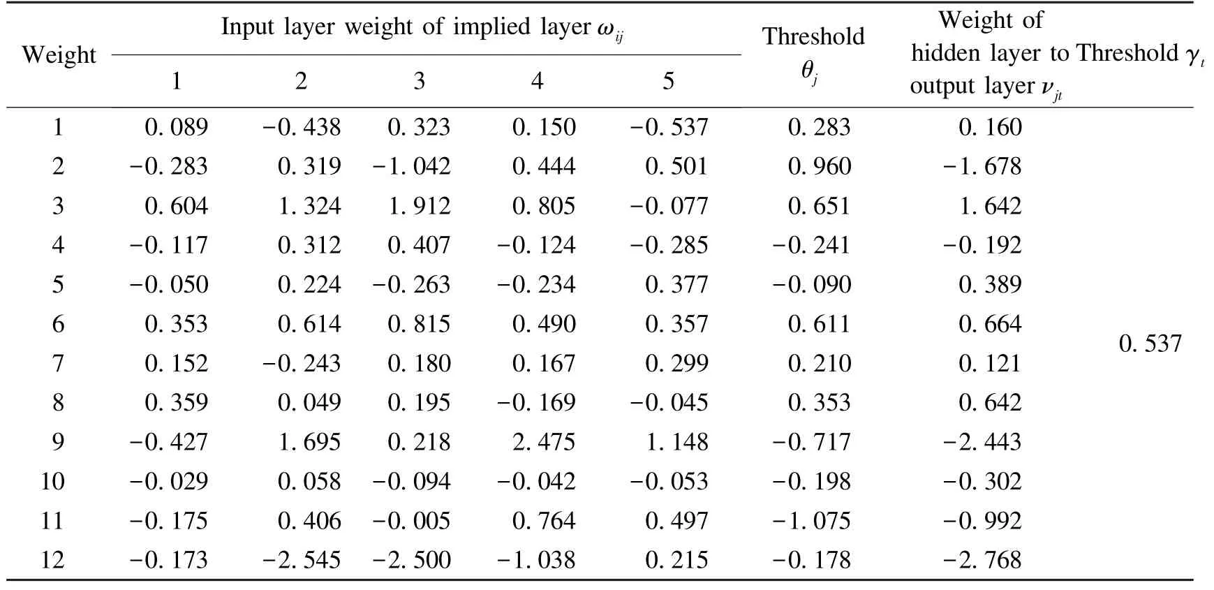
Table 6 Weights and thresholds(compression modulus)

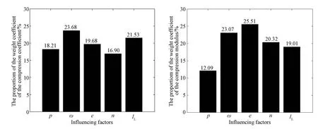
Figure 5 Weight coefficient of each factor(total=100%)

It can be seen from Fig.5 and Fig.6 that the two neural network models have a good generalization ability for the mapping relationship between the compressibility parameter and the nonlinear function of the selected parameter,but there is still a certain gap between the two in terms of output accuracy.In the compression coefficient model,the correlation coefficient between the output value of the Bayesian regularized neural network and the target training value reaches 0.999,while the correlation coefficient between the output value of the traditional LM-BP neural network and the target training value is 0.956.In the compression modulus model,the correlation coefficient between the output value of the Bayesian regularized neural network and the target training value reaches 0.997,while the correlation coefficient between the output value of the traditional LM-BP neural network and the target training value is 0.905.Therefore,compared with the traditional LM-BP neural network model,the output of the BR-BP neural network model is more stable and the correlation is higher.

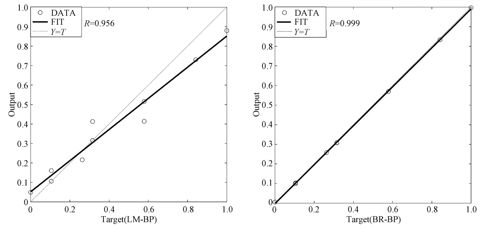
Figure 6 Comparison of fitting results of two models(compression coefficient)

Figure 7 Comparison of fitting results of two models(compression modulus)

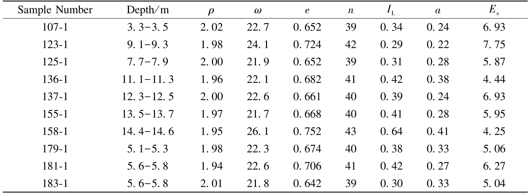
Table 7 Verification samples

The output error curve of the validation sample data is shown in Fig.8:

Figure 8 Error curve

2.3 Model Testing and Error Analysis

After the network training is completed,the established Bayesian regularized neural network is simulated through the measured data.Meanwhile,the output of the network is obtained by using the simulation function.By comparing whether the error between the output value and the measured value meets the requirements,the network's generalization ability is checked.The test data are shown in Table 8:

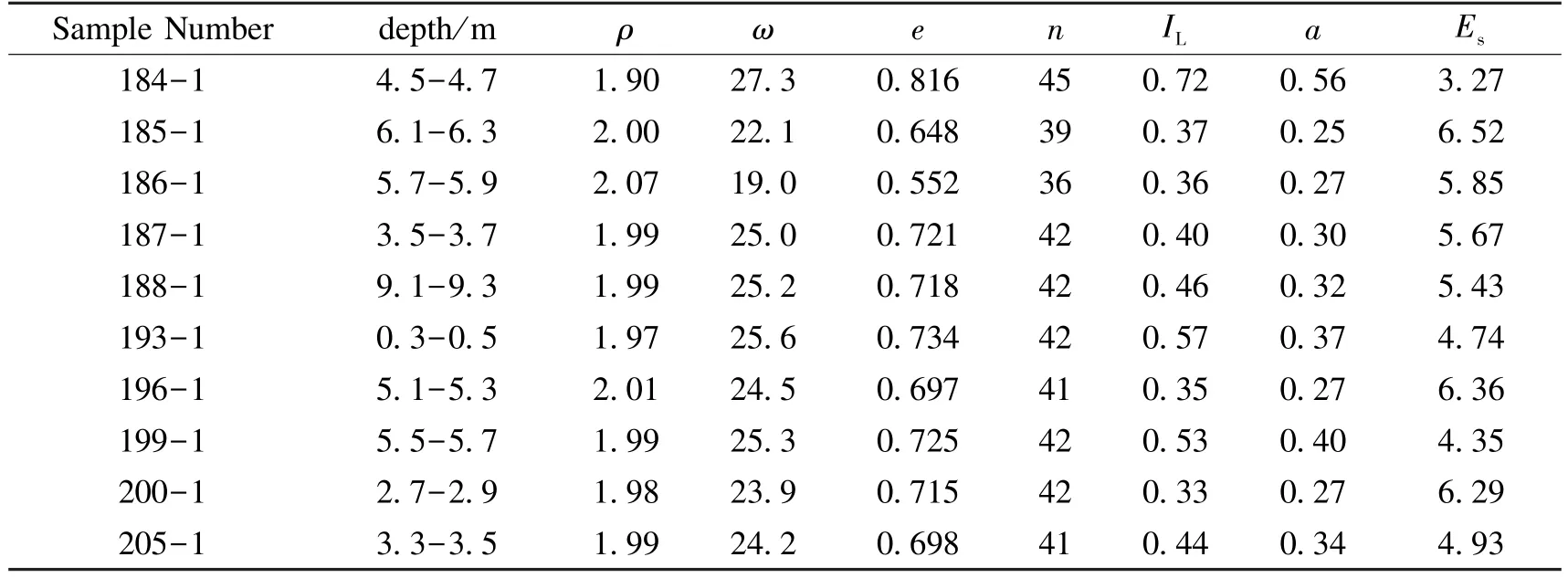
Table 8 Testing Data

The output results of the two neural networks are shown in Table 9 and Table 10.It can be seen from the tables that the maximum absolute error and relative error of the compression coefficient output by the LM-BP neural network model are 0.16 and 64%,respectively.The average value of the relative error is 15.54%;The maximum absolute error and relative error of the compression coefficient output by the BR-BP neural network model are 0.08 and 29.6%,respectively.The average relative error is 6.15%;the maximum absolute error and relative error of the compression modulus output by the LM-BP neural network model are 2.28 and 39.0%,respectively.The average relative error is 6.07%;The maximum absolute error and relative error of the compression modulus output by the BR-BP neural network model are 1.70 and 29.1%,respectively.The average relative error is 4.62%.Such results show that the model is more stable and has better advantages in solving nonlinear problems such as high dimensionality.

Table 9 Output results of different neural network models

Table 10 Output results of different neural network models

In order to reflect the accuracy of the output results of the two neural networks more intuitively,the output results of the two neural network models are superimposed and compared,as shown in Fig.9 and Fig.10:

Figure 9 The output results(a) and error curve (b)

The errors of the output results of the two models according to Fig.9 and Fig.10 are both acceptable,indicating the applicability and effectiveness of the compressibility parameter study.LM-BP neural network has excellent autonomous learning ability and strong generalization ability.This paper utilizes the advantages of LM-BP neural network and solves the problems existing in traditional LM-BP neural network,then proposes a Bayesian regularization BP neural network output model,and finally compares it with the traditional BP neural network output model.Overall,the traditional BP neural network output model is prone to fall into local minimization,while the BP neural network output model after Bayesian regularization improves the local minimization problem obviously.The relative error of the output is small.The BP neural network output model after Bayesian regularization is more stable than the traditional BP neural network output results,indicating that the BR-BP neural network is more suitable for the output of the compressibility parameters of silty clay in the study area.

Figure 10 The output results and error curve ( Es)

3 DISCUSSION AND CONCLUSIONS

The compressibility parameters of silty clay are affected by various factors,and the nonlinear mapping between them and variables is difficult to be represented by an accurate mathematical function model.Therefore,based on the experimental data,the paper uses correlation analysis (SPSS) and Bayesian regularization neural network to establish the output model,the following conclusions are obtained:

(1)Most of the silty clay in the study area is medium compressive,and there is also high compressive silty clay.However,the accidental results of the test are not ruled out.As can be seen from the output of the paper,the test result is a sample of highly compressive silty clay.Furthermore,the output result based on the BR-BP neural network model is still highly compressive silty clay,indicating that the results of this sample are not associated with test errors.

(2)The correlation analysis method is used to select the main influencing factors with high correlation,and replace all the original variables as input parameters to build the model.This method effectively reduce the dimensionality,eliminate the information redundancy between variables,and significantly improve the training efficiency and output accuracy.

(3) According to Garson theory,among the factors affecting the compression coefficient of silty clay in this area,ωandILare relatively prominent.Among the influencing factors of compression modulus,eandωare larger,while the proportion ofρis smaller.

(4) The inspection of the measured data and the comparison with the unimproved BP neural network model are both excellent,indicating a relatively stable output of the model.In detail,the average value of the relative error of the compression coefficient is reduced from 15.54% to 6.15%,the average value of the relative error of the compression modulus is reduced from 6.07% to 4.62%,and the accuracy of the output results is significantly improved.When this method is applied in practice,the workload can be effectively reduced compared to the experimental workload.Besides,the efficiency is high and the accuracy can also meet the relevant requirements.It shows that the research method has good theoretical significance and practical value,and provides a new technical method for obtaining the compressibility parameters of silty clay in this area.