Application on Anomaly Detection of Geoelectric Field Based on Deep Learning1

WEI Lei ,AN Zhanghui* ,FAN Yingying ,CHEN Quan ,YUAN Lihua and HOU Zeyu

1)Lanzhou Institute of Seismology,China Earthquake Administration,Lanzhou 730000,China

2)Lanzhou Geophysics National Observation and Research Station,Lanzhou 730000,China

3)Gansu Earthquake Agency,Lanzhou 730000,China

4)School of Science,Lanzhou University of Technology,Lanzhou 730050,China

The deep learning method has made nurnerials achievements regarding anomaly detection in the field of time series.We introduce the speech production model in the field of artificial intelligence,changing the convolution layer of the general convolution neural network to the residual element structure by adding identity mapping,and expanding the receptive domain of the model by using the dilated causal convolution.Based on the dilated causal convolution network and the method of log probability density function,the anomalous events are detected according to the anomaly scores.The validity of the method is verified by the simulation data,which is applied to the actual observed data on the observation staion of Pingliang geoeletric field in Gansu Province.The results show that one month before the Wenchuan MS8.0,Lushan MS7.0 and Minxian-Zhangxian MS6.6 earthquakes,the daily cumulative error of log probability density of the predicted results in Pingliang Station suddenly decreases,which is consistent with the actual earthquake anomalies in a certain time range.After analyzing the combined factors including the spatial electromagnetic environment and the variation of micro fissures before the earthquake,we explain the possible causes of the anomalies in the geoelectric field of before the earthquake.The successful application of deep learning in observed data of the geoelectric field may behefit for improving the ultilization rate both the data and the efficiency of detection.Besides,it may provide technical support for more seismic research.

Key words:Deep learning;Time series;Dilated causal convolution;Geoelectric field;Abnormal detection

INTRODUCTION

Geoelectric field anomalies may be associated with all stages of the preparation process of an earthquake.(Varotsos P.et al.,1984;Meyer K.et al.,1986;Nagao T.et al.,1996,2000;Mogi T.et al.,2000;Uyeda S.et al.,2002;Ramírez-Rojas A.et al.,2008;Orihara Y.et al.,2009,2012;Huang Qinghua et al.,2006;Fan Yingying et al.,2010,2014,2015;An Zhanghui et al.,2011,2013;Liu Jun et al.,2011).In order to explain the observed anomalies,researchers have conducted experimental simulations on the basis of theoretical mechanisms (Dobrovolsky I.P.et al.,1989;Guo Ziqiang et al.,1988,1995,1999;Hao Jinqi et al.,2003;Huang Qinghua et al.,2006;Du Xuebin et al.,2007,Du Xuebin,2011;Gao Yongxin et al.,2009;Tan Dacheng et al.,2010,2012).The aforementioned previous studies indicate that it is extremely beneficial for the earthquake prediction research if the anomalous seismic information can be extracted from the geoelectric field data efficiently.Therefore,a method for extracting information from the geoelectrical field anomalies is particularly important.

With the rapid development of artificial intelligence,researchers at home and abroad have introduced several methods which include independent components analysis (ICA),principal components analysis (PCA) and neural network to extract the geoelectric field information prior to an earthquake.Orihara Y.et al.(2009) investigate the feasibility of extracting the size of the abnormal variation from the daytime noise data of the geoelectric field station using ICA.With the support of the statistical characteristics of the actual seismic signal,Li Hong et al.(2010) also use ICA to achieve the separation of the effective signal and noise.Telesca L.et al.(2004) utilize the PCA method and find that an increased pre-seismic principal component may appears as a seismic precursor,revealing the PCA is an effective method for processing geoelectric field data.Han Peng et al.(2009) also use PCA to extract relatively weak seismic geomagnetic information from stronger background interference.Combining neural networks,Hilbert transform with the proposed signal processing algorithm,Kanarachos S.et al.(2017) detect anomalies in geomagnetic field signals for predicting seismic activities.Qiu Hongmao et al.(2005) use neural networks to effectively classify seismic signals Qiu and obtain positive results.

The method of deep learning for seismic signal anomaly detection in this paper is developed on the basis of artificial neural networks.With the increasing development of artificial neural networks,deep learning has become one of the most popular methods.The uniqueness of deep learning is due to the ability to automatically learn advanced features relevant to seismic anomaly predication.It is able to intelligently distinguish and capture anomalous noises in the geoelectric field data with little manual selection and related expertise.In this process,it takes into account both the stochastic and temporal nature of a seismic event,and has a strong ability to approximate real-valued functions and learn the functional relationships of seismic events over time for the purpose of making effective predictions of anomalous events.

The deep learning method for time series anomaly detection mainly include two steps:(1) Constructing and analyzing a deep learning model for the future trend prediction.The example is selected as the 2008-2013 time-average value of the NE track of Pingliang geoelectric field and the training set is the denoised data.(2) Using the difference between the predicted and real values as the prediction error,calculate the mean and variance of the prediction error,then combining the probability density function to calculate the log probability density value as an anomaly score,and using this as a criterion to monitor the abnormal events to analyze their correlation characteristics.

1 NEURAL NETWORK MODEL

1.1 Dataset

The data from the Pingliang observatory have been usually applied to the WenchuanMS8.0 earthquake and YushuMS7.1 earthquake and the study of tidal variations in the geodetic field repeatedly.The Pingliang geoelectric observatory adopts the “inner triangle”polar distribution method.The time-averaged points of the long polar distance NE channel of the Pingliang observatory from January 1st,2008 to June 30th,2010 based on the waveformprocessing software and physical analysis method are converted into CSV files as experimental data.Particularly,the 2009 data are selected as the training set and a 20%cross-validation is set for a total of 8 760 time mean points.There are no apparent earthquakes around the station during the training set.Finally,a total of 13 140 data points are used to construct the neural network model.

1.2 Wavenet Model

Before constructing the Wavenet model,we perform preprocessing operations on the above data set.Firstly,singular spectrum analysis (SSA) method is utilized to denoise the data from Pingliang observatory.Here,the denoised data are normalized and scaled,then the data of the time-averaged points are converted into supervised data in machine learning.The set of the time-averaged points is a series of numbers ordered by time index,and the supervised learning data set consists of input modexand output modey.From the input mode to learn how to predict the output mode,this is equivalent to creating the lagged observations of each column and the precursor observations,transformed to the supervised learning data format.The original time series is then subjected to a first-order differential for the purpose of eliminating some fluctuations and smoothing the data series.

The Deep Mind Company of Google has published a speech generation model of WaveNet.Due to the similarity with the data structure,we apply the WaveNet to generate the time series of the geoelectric field.After preparing the data set,we start to establish the Wavenet model,which is shown in Fig.1.

The Wavenet model whose main block is the dilated causal convolution,uses residual networks and skip connections in its structure to accelerate convergence.The residual network uses a skip connection with thek-layer network.During the computation,168(7-days) time-averaged points are input initially.After using causal convolution method,the expansion convolution is performed in the hidden layer and enters the residual unit,in which each residual net has two paths.The geoelectric time-average value are directly as the input of next residual block after the constant mapping and ReLU,and finally output by jump connection.The predicted outputp(xt|x1,x2,x3,…xt-1) of the model at momenttdoes not depend on the dataxt+1,xt+2,…xt+nfor any future moment but only related to the time-averaged value of the geoelectric field before momentt.Furthermore,the output at thetmoment is a distribution ofxt,the distribution parameterθcan be obtained by maximizing the following likelihood function (Equation (1)):

During the process of model training,the predictions for each node are computed in parallel,and the output of each point is fed back into the model as a new input.While making the prediction,whenever a new time-averaged point of the geoelectric field signalxtis predicted,it immediately input the signal sequence about the next nodext+1.Twenty-four(1 day) time-averaged points are predicted as the time-averaged points of the eighth day,and then 24 points (the time of one day) are used as the step length.A total of 8-day data from the original input day 2-8 and the new forecast data from day 9 will be used as the new input.The fixed time length is controlled by a sliding window as the control condition for the time series.Similarly,the new sliding window is shifted backward for the calculation of the next day,and the predicted sequence is generated after analogy.During the calculation process,WaveNet is able to capture the features of the time series of the geoelectric field with strong fidelity and contain seismic-related time series information.Finally,a sequence that is highly consistent to the actual geoelectric field data is generated.

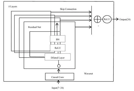
Figure 1 The model structural diagram of Wavenet

1.2.1 Dilated Causal Convolution

The dilated convolution is the method for obtaining a larger receptive field by adding the dilation rate.It also allows the use of more historical data by superimposing several layers of the dilation convolution in order to extract long-term patterns in the time series of the geoelectric field.The causal condition is introduced in the causal convolution model to extract short-term patterns in the sequence and to better extract necessary information implied by the sequence.To avoid the violation from the modeling order of the data,the predictions issued by the causal convolutional model can only rely on the present and previous time series.Dilated convolution is a convolution in which the filter skips the input value in a specific step,thus allowing a larger range of data information to be obtained(Chen L.C.et al.,2014),and consequently increasing the perception level of the model.In addition,dilation rate is added into the traditional convolution kernel in this paper.We setlk-1as the size of the receptive field of the layerk-1,fkas the size of the convolutional nucleus of the current layer,andSito be the step length of layeri.Here,we sample the original input image at intervals of expansion rate minus 1.For the convolutional nucleus itself,it is equivalent to insert a zero inside a convolutional nucleus that has not been convolved using a hole.Therefore,the size of the convolutional nucleus that is convolved with the original image becomes larger after using the hole convolution.The expansion rate of the three hidden layers [1,2,4],the step length of each layer is uniformly set to 1,the size of the convolutional nucleus is 2,and d stands for the Dilation rate in each layer.The parameter d is added to obtain the relationship between the sensory fields in each layer as shown in Equa.(2).It is calculated that the size of the Wavenet receptive field is 7.

The dilated convolution increases the receptive field without the loss of feature map size after increasing its internal complement with 0,However,it also brings new problems.As the input of the training data,a discontinuity of convolutional centroids appears in the overall feature map.The possible reason is that the convolutional nuclei are spaced,leading to an incompletion in data points for calculation.Such situation occurs especially when the superimposed convolutional layers are processed with the same dilation rate.Therefore,if we use different,continuously arranged expansion convolution in the model and set the“jagged” expansion rate with three hidden layers [1,2,4],then the distribution of convolution centers will not be missed.In this way,the dilation convolution and the causal convolution can jointly form the causal dilated convolution (Van den Oord et al.,2016).

1.2.2 Residual Network

A residual network is a type of network that is optimized and designed for deep learning.A deep neural network generally refers to a neural network consisting of more than five layers of adaptive nonlinear units.Among them,each layer contains a large number of trainable parameters.The network approximates the intrinsic nature of the input data through the combination of these nonlinear structures and the training of parameters.However,as the layers deepen,several problems may appear,such as gradient disappearance.He Kaiming et al.(2015) propose a residual network model that overcomes the problem of gradient nonconvergence of the deep network,ensuring the training effect of the input ground electric field signal in the network.This model solves the problem of gradient disappearance and improves the performance of the network by simply increasing the network depth.Consequently,the nonlinear relationship of the actual geoelectric field signal is delineated preferably.Here,the structure of the residual elements of the constituent units of the residual network is shown in Fig.2.

Among them,BN represents batch normalization,which can further avoid the signal attenuation as the layers deepen,reducing the instability of the training process.As can be seen from the figure,unlike the single-path signaling structure of a normal neural network,in a residual network,in addition to the normal passage of the input signal through the network layer,there is a direct connection between the input and output sites that makes up the residual structure.This jump connection can provide a constant mapping to calculate the residual of this output.We equate the traditional network training fitting function (x) to the finding residual (x)-xfitting function (x).In addition,the forward process of the residual network is linear,and the average ground-field-time in the next layer is equal to the constant mapping of the variables plus the result of the residual mapping in the residual element,thus having an absolute computational advantage.The output is calculated as follows;

wherexl+1is the output corresponding to the inputxl+1at layerlandwlis the weight at layerl.

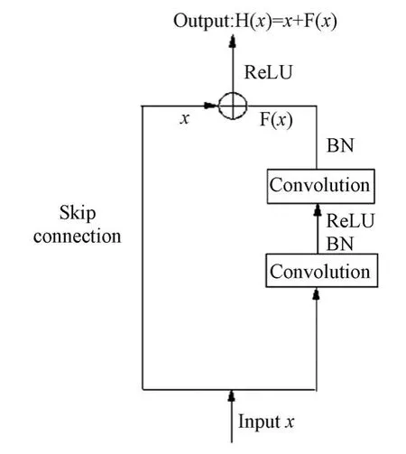
Figure 2 Residual network structure diagram

1.2.3 Loss Function

The loss function is used to estimate the degree of the inconsistency with the true value.This paper adopts Huber loss (Huber loss) as a loss function (Equa.5),which has the advantage Compared with the mean square error loss function.Huber loss is less sensitive to possible interference in the training data.Such robust loss can learn the normal information implied in the training.In addition,compared with the mean absolute error loss function,there is no non-inducible Huber loss in backward transfer process of the model.

whereydenotes the time-averaged value received by the real station,f(x) represents the predicted value,andδis the tuning-constant parameter.The mean absolute error loss function is used when,and the mean absolute error loss function is used when;and the Huber loss function is more robust to anomalies whenδis smaller.In this paper,we choose the appropriate parameterδbased on the results predicted by the model.Huber loss is actually a compromise between MSE and MAE because it defines a parameterδwhose main role is to judge whether a data point is an outlier or not.When our predicted value is far from the true value,we choose Mean Square Error (MSE).Conversely,we use Mean Absolute Error(MAE),instead.For the initial values,we set theδvalue to 1,epoch is 6 000,and train the model using Adam optimizer.We also set the batch size to 128 and initialize the network weights using normal distribution initializer.When the training is stable,the loss reaches 0.4.In this process,we need to iteratively adjust the hyperparameterδ.In the end when theδvalue of 0.35 is selected,the model loss is further reduced,and in this process we use early stopping and dropout to prevent network overfitting,and in the end the loss is reduced to 0.2 when it is stable.

1.3 Evaluation

In this paper,three methods of error measures are chosen to evaluate the predictive performance of the model.Before Equa.(5),we conduct normalized treatment to ensure the morphological variation of the data and the comparability between the indicators for the purpose of obtaining a better assessment of the effectiveness.

wherex,x′,xmax,xminrepresent the original value,pre-processed obtained value,maximum value,and minimum value of the signal,respectively.

Root Mean Square Error (RMSE),Mean Absolute Error (MAE),and Correlation Coefficient (CC) of the true value ofxand the predicted value ofx′for a time series with a sample size ofN,are shown in Equa.(6),(7) and (8),respectively.For root mean square error and mean absolute error,smaller calculated values indicate better prediction by the model.However,for correlation coefficients,highervalues indicate better prediction.The coefficients for evaluating the predictive performance for the relevant data set are shown in Table 1.

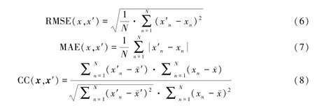
Table 1 Model Performance Evaluation Coefficient Table

2 ANOMALY DETECTION

This paper uses an anomaly detection model based on log probability density to detect earthquake.Firstly,we establish a model to detect anomalies which have poor fitting results.For example,a data distribution model can be created by estimating the parameters of the probability distribution.If an object does not obey the distribution,it is considered an anomaly.Under the assumption of a normal distribution,if there is a new sample,the region ofμ-3σ ≤x≤μ+3σ contains the vast majority of the data.Then we select two points A and B as boundary points for anomaly detection.We consider the section wherexis less thana1and greater thana2is an anomalous section,at which point the probability density value is ε.Therefore,this sample can be considered anomalous when the normal distribution value ofx,the probability density value,is less than the thresholdε.The calculated error setX={x(1),x(2),...,x(m)} is able to recognize if a sample is anomalous by the following function:

wherex(i)is known,μandσare estimated by maximum likelihood.We compare the calculated value with the ε value.If it is less than ε,it is considered an outlier,which will be further processed using logarithm.The values greater than the median are reduced by a certain percentage using logarithm,leading to smoother time series and better data which resembles a normal distribution.According to the central limit theorem,when a large number of independently random variables are added,their normalized sun tends to be a normal distribution.The log-normal distribution is a type of transition distribution between extreme and normal distributions,and the log probability density errors are often used in financial stock predictions,and detection of anomalies in geological phenomena.Therefore,we perform a log transformation (log(x)) and a Shapiro test on it after taking the logarithmic treatment for better statistical inference and anomaly detection.

The logarithmically processed data are shown in Figs.3 and 4,where the blue dots represent seismic anomalies.we select earthquakes with magnitude greater than or equal to 6.0 for the corresponding time period in the study below.The results indicate that after taking the logarithm of the sample error,the smoothness and differentiation of the series are better in 2008 and mid-June,2010.Also,there is a constantly steady state over a period of time.The sample has a significantly reduced peak co-transit compared with the preceding logarithm.The bias distribution is also significantly reduced,resulting in a smaller variance.In addition,the Shapiro test is performed after logarithmic treatment and the results suggest that the P values of the time-averaged points are close to 0.05 and the data in local time period are closer to the regularity of normal distribution.Therefore,anomaly detection by the log probability density method after transformation is a more effective method for the anomaly detection in this paper.

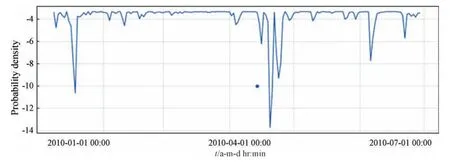
Figure 3 Logarithm of sample error in 2008

X1,…,Xnis the error of the average time for each geoelectric field and the overall distribution of the error isf(X;θ1,…,θk) .Whenθ1,…,θkis fixed and treated as a function ofX1,…,Xn,L is a probability density function.Thus,if log((Y1,…,Yn;θ1,…,θk))＞log((X1,…,Xn;θ1,…,θk)),(X1,…,Xn) will occur less likely at the time of observation than(Y1,…,Yn) .A lower log probability density value indicates a lower probability of error,and the corresponding point is an anomaly.On the contrary,when the log probability density value is large and stable,the corresponding data is normal.

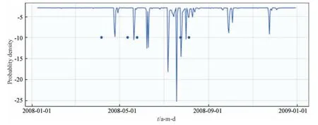
Figure 4 Logarithm of sample error in 2010.01-2010.06

To test the validity of the methods and exclude the effects of anomalous signals caused by noise,the discrete data sequences required for the analysis (sample size 4713) are generated using Equa.(10).The simulated data and noise signals contained 24 hr,12 hr,and 8 hr period components similar to the geoelectric field (gaussian noise with a mean value of 0 and standard deviation of 0.7).The anomalous data points are marked as red dots in Fig.5.The simulated signal is handled using normalized processing method,which can ensure the morphological changes of the data and avoid excessive loss of information for the purpose of facilitating a better model training.The outliers here are all in the test set (noted as test set 1).

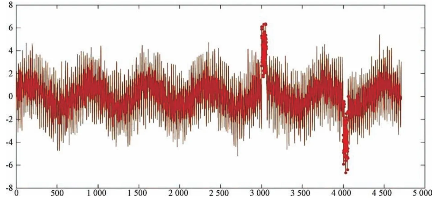
Figure 5 Analog signal diagram

Fig.6(a) gives the results of the model's predication for test set 1.From the predictive performance evaluation coefficients (Table 1),it can be seen that the model predicts well for set 1.For individual normal data points the anomalies in the predictions are false due to anomalous information in the sequence.In order to suppress the prediction error,24 data errors and anomaly prediction detection are selected and the total error sums were divided into 74 groups.With the group number being 4,5,6,46,47,48,the logarithmic probability density curve of the corresponding error is shown in Fig.6(b).It can be seen from Fig.6(b) that shows the logarithmic probability density value of the error corresponds to the abnormal group number each time when it suddenly decreases.Besides,the normal group number is more stable,indicating that the log probability density value of the error can reflect the normal perfectly.

In summary,the availability and validity of the expanded causal convolutional model and the log probability density function method for the detection are verified by simulation experiments.Meanwhile,the effect of interference signals on the detection of anomalies is excluded.

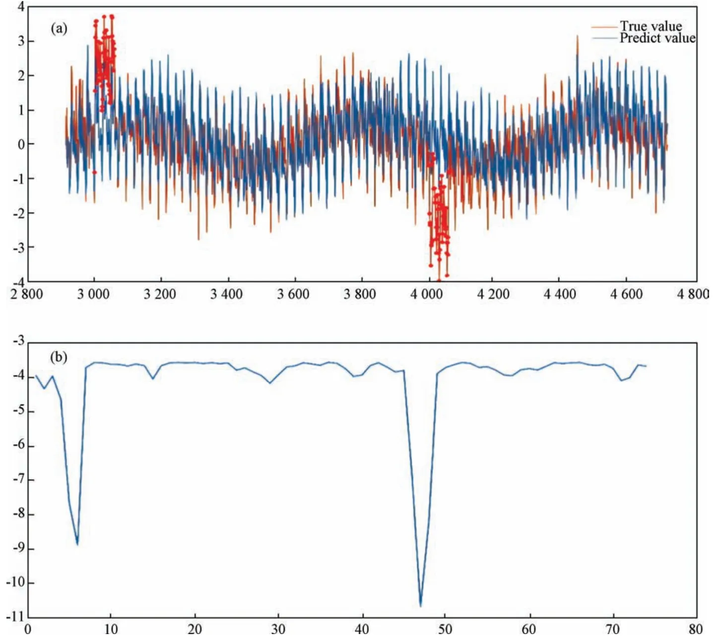
Figure 6 (a)Test set 1 prediction map;(b)Test set 1 log probability density map

3 ANALYSIS OF PINGLIANG STATION

The Pingliang geoelectric field observatory (35°90′N,106°93′E) is situated at the eastern edge of the Qilian fold belt,west of the Ordos Basin,and south of the inland Heilan-Liupanshan formation belt,the location that is the intersection of several different tectonic complexes(Fan Yingying et al.,2014).The geological structure of the area around the station is complex and earthquake activities occur frequently.The observations and analyses from Pingliang station have been applied to the study of the WenchuanMS8.0 and YushuMS7.1 earthquake,as well as the research of tidal variations in the geoelectric field.(Tan Dacheng et al.,2010,2012;An Zhanghui et al.,2013;Fan Yingying et al.,2014).

After analyzing the anomalies of the pre-earthquake geoelectric observations,Zhang Xuemin et al.(2007) propose that the range of geoelectric field anomalies is related to the gestation region,indicating that the range of pre-earthquake geoelectric field anomalies can be estimated from the range of gestation region.The range of the gestation zone is estimated usingr=100.43M,whereris the radius of the gestation zone (km) andMis the magnitude(Dobrovolsky I.P.et al.,1979).In this paper,the seismic events that may have influenced the data from 2008 to 2013 in Pingliang station are selected using the pregnancy zone range estimation method,as shown in Table 2.The relevant times in the paper are all expressed in Beijing time (UTC+8).

Table 2 Earthquakes around Pingliang Station with MS ≥6.0

3.1 Anomaly Detection of Pingliang Station

In order to exclude the effects of the interfering signals,we all use the denoised data as experimental data.Here,the average time of the long polar distance NE trajectory from January 1st,2008 to June 30th,2010 are used as the experimental data.Besides,the data from the first six months of 2009 are used as the model validation set and those from the last six months are utilized as the training set.The training set corresponds to a time period in which there are no earthquakes around the station,and the dilated causal convolutional network can learn the normal information implied by the data from the training set for model construction.The data from January 1stto December 31st,2008 and January 1stto June 30th,2010 are used as the model test sets,which are recorded as test set 2 and set 3.Fig.7(a)and 7(b) show the prediction results of test sets 2 and 3 respectively,and Table 1 shows the prediction performance evaluation coefficients for the corresponding test sets.

Fig.8 shows the log probability density plot of daily cumulative errors for the test sets.Fig.8(a) shows that the log probability density values of the daily cumulative errors of the model prediction from January to April 2008 are stable and at high values,thus the observations are normal during this period.In Fig.8(a),the corresponding earthquake event is WenchuanMS8.0 earthquake,WenchuanMS6.2 aftershock,and WenchuanMS6.3 aftershock.The earthquake event in Fig.8 (b) is the YushuMS7.1 earthquake.The vertical coordinates represent the log probability density values.In the first month before the WenchuanMS8.0 earthquake and its 2 aftershocks,the log probability density value decrease significantly compared with the previous 3 months,indicating anomalies may appear in the observations at the corresponding time.In Fig.8(a),the log probability values of the model prediction errors in late April,late May,mid-July to mid-August and early October 2008 show large changes,with the minimum values reaching -9.Furthermore,the corresponding observations exhibit stepwise abnormal changes,while the log probability density values of the model prediction errors in other time periods are in the range of -2 to 0 with no significant changes.

Figure 7 Test set 2 prediction map (a) and Test set 3 prediction map (b)

Then we take the log probability density value as an anomaly score.Based on the value of the log probability density in the test set of Pingliang Station,we set the ε threshold to-6.The values of log probability density less than -6 are considered as anomalies,which indicates that the probability of model prediction errors occurring in this time period is extremely low and there are anomalies in the observations of the corresponding time period.A value greater than -6 is considered to be in the stable range,i.e.,normal observations at this time.It can be seen from Fig.8 that the anomaly detection based on this method is conducted to match the corresponding seismic event in the Fig.8.

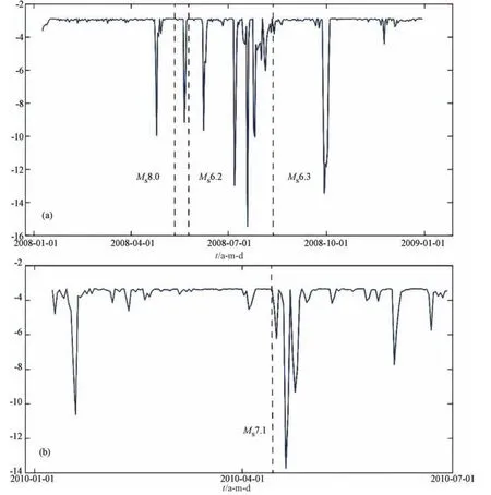
Figure 8 (a) Logarithmic probability density map of daily cumulative errors of test 2;(b) Logarithmic probability density map of daily cumulative errors of test 3

Similar to the process described above,the time-average values of the NE long-pole distance measurements at Pingliang geoelectric field station in 2012 and 2013 are analyzed.Similarly,the first six months of 2012 are selected to form the model validation set and the second six months to form the training set.The data from January 1stto December 31st,2013 are used as the model test set and denoised and recorded as test set 4.According to Fig.9,the model fits well to the predicted results of test set 4 and the predictive performance evaluation coefficient in Table 1.

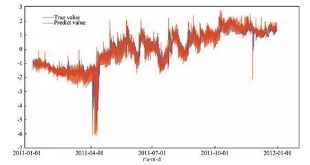
Figure 9 Prediction map of Test set 4

Fig.10 shows the log probability density plot of daily cumulative errors for the test set.As can be seen from Fig.10,The two corresponding anomalies are the LushanMS7.0 and MinzhangMS7.0 earthquakes.The log probability density values of the daily cumulative errors of the model are relatively stable between January and February 2013,thus there are no anomalies in the observations for this period.The prediction value for the first month before the LushanMS7.0 and MinzhangMS7.0 earthquakes suggests a descending trend of anomalies.In addition,the log probability density value of the daily cumulative error of the model prediction value is also unstable during the aftershocks of the Lushan earthquake,indicating anomalous information.

Figure 10 Test set 4 daily cumulative error logarithmic probability density map

3.2 Result Analysis

Here we relate the detected anomalies to the anomalous mechanism of the pre-seismic electromagnetic field.In laboratory simulations of rock fracture,it has been observed that rock fracture may excite low-frequency electromagnetic signals and the decrease of resistivity.(Guo Ziqiang et al.,1988,1995,1999;Hao Jinqi et al.,2003) These findings provide an experimental basis for the observed seismic electromagnetic phenomena.However,the signal generation mechanism of the pre-seismic electromagnetic field is still equivocal.

Geoelectric field measurement mainly includes two components,measurements from geodetic electric field and natural electric field.In detail,geodetic electric field is the induction of various current systems in the Earth's internal medium in outer space,while natural electric field is mainly the local phenomenon caused by the physical and chemical processes in the Earth's internal medium.Ground-field observation data are heavily influenced by the electromagnetic environment in space,and magnetic effects need to be taken into account in data analysis.We consider that ∑Kp ＞30 is an indication of strong geomagnetic activities,and if the Dst index is below -30 and lasts for more than 2 hours,a magnetic storm may occur.

In addition,changes in natural electric fields prior to the earthquake may also cause such anomalies.It is generally accepted that natural electric fields are produced mainly in the redox mode,diffusion mode and subsurface fluid seepage filtration mode of the ore body.In studies related to earthquakes and volcanic eruptions (Adler P.M.et al.,1999;Ishido T.et al.,1996),diffusion patterns and seepage filtration patterns of subsurface fluids are more acceptable.During the late gestation period,an avalanche-like increase in microfissures within the subsurface medium may occur due to tectonic stress(Mjachkin V.I.et al.,1975;Mei Shirong et al.,1993).These newly generated micro fissures are interconnected to cause the migration of subsurface fluids,and the electric field formed by the movement of charged particles in the subsurface fluid may disrupt the stable natural electric field,providing a possible explanation for the anomalies detected in the paper.For the Pingliang Station,if the station's rocky structure changes before an earthquake,it is possible that it will be observed in the geoelectric field observations.In addition,An Zhanghui et al.(2013) and Tan Dacheng et al.(2010) detect the waveform variation of the geoelectrical signal waveform from April 24thto 26thbefore the WenchuanMS8.0 earthquake,using dominant period method.The results are generally consistent with the time of the log probability density anomaly detected in this paper from April 23rdto 26th.Liu Jianbo et al.(2014) measure the ratio of geodynamic field length to short polar distance from 39 geoeletrical field stations near the epicenter of theMS7.0 earthquake in Lushan.They also find that most of the anomalies of ipsilateral polar distance occurred about half a year before the earthquake are similar to the results in this paper.Fan Yingying et al.(2013) detect a large anomalous fluctuation in the geoelectric field of the long polar distance gauging channel in Pingliang Station before the Minxian-Zhang xianMS6.6 earthquake.At the same time,the seismic power spectral density in Pingliang Station also shows a continuous increase in the 50 days before the 2010 LushanMS7.0 earthquake.The results are basically consistent with the anomalous time of the pre-log probability density values of the Lushan earthquake detected in this paper and shown in Fig.7.In addition,the neural network model exhibits a strong ability to approximate real-valued functions,taking into account both the stochastic and the temporal nature of seismic occurrence.Besides,it predicts new seismic signal samples that can achieve convenient and efficient purposes,avoiding complicated process of manual selection and calculation.Deep learning networks can easily learn the functional relationships that may change over time as a result of seismic events,providing effective prediction of anomalous events.

Figure 11 Geomagnetic ∑KP index map from 2008 to 2013 (a)Dst index map from 2008 to 2013 (b)

4 CONCLUSION

Based on the introduction to the theory of dilated causal convolutional model in deep learning and how to use the method for modeling and anomaly detection,the effectiveness of dilated causal convolutional networks in processing time-series anomaly detection is verified through the simulation of experiments.Then,the data from Pingliang geoelectric field station is analyzed and several meaningful conclusions are obtained as follows.

(1) Based on the analysis of the simulated time series data and the real observations from Pingliang Station,it can be seen that the model can effectively extract the characteristics from the observations,and it also proves the applicability of the construction method to the observations.

(2) The log probability density values of daily cumulative errors predicted by the deep learning method for the Pingliang data shows a sudden decrease during the first month before the WenchuanMS8.0,LushanMS7.0,and MinzhangMS7.0 earthquakes.Among them,before the WenchuanMS8.0 and LushanMS7.0 earthquakes,the deep learning method is able to detect anomalies that might be related to the earthquakes,and the results of the study are largely consistent with those provided by previous authors.

(3) The application of the deep learning method to the electric field data and anomaly detection analysis has plenty of advantages,including automation,high-precision processing and concise analysis results.Besides,the model is more stable in processing large amounts of seismic data.

Automated and intelligent processing of seismic precursor data is an important component of seismology.It also represents the innovation of engineering technology and is consistent with the future development trend.The neural network described in this paper implements an end-to-end intelligent model that integrates prediction,anomaly detection,and anomaly reporting,providing some new research methods for the development of artificial intelligence in the field of earthquake prediction.Additionally,new ideas and insights can be discovered by earthquake researchers and earthquake workers using the method.Meanwhile,since the method is still in the development stage,the theoretical foundation and the specific analysis process are needed to be improved,and the role of the detailed parameters is needed to be further understood for the purpose of building a better model.The results of the analysis still have some logarithmic probability density anomalies that don't correspond to seismic events.Therefore,more selection method of seismic events,as well as more information on seismic cases are still needed for retrospective testing.

ACKNOWLEDGEMENT

The geoelectric field observations used in this paper are from national earthquake precursor networks center.We would like to express our gratitude to the staff of the station for their hard work and to the editorial teachers and experts for their valuable suggestions.