相关噪声驱动下一种特殊非对称非线性系统的随机共振研究

范泽宁，李鹏飞，陶原野，唐一弓，邓 科

(1. 四川大学数学学院，成都 610065； 2. 平安银行股份有限公司博士后工作站，深圳 518000；3. 四川大学生命科学学院，成都 610065)

1 Introduction

The original work on stochastic resonance by Benzietal.[1]in 1981，in which the term was coined，was in the context of modeling the switching of the Earth's climate between ice ages and periods of relative warmth with a period of about 100 000 years. From 1983 to 1989，Pesqueraetal.[2-3]analyzed this type of non-Markovian processes in terms of a path integral formulation is rare up to recent times. In 1989，Presillaetal.[4]came up with the famous adiabatic approximation theory successively. From 1989 to 1991，adiabatic perturbation theory was put forward by Jung and Hanggi[5-6]，that provides a necessary theoretical basis for the study of stochastic resonance. At the present stage，the study of stochastic resonance under complex system and complex noises is helpful to feature extraction and detecting weak signal of high-precision machinery at low SNR situation[7-9].

Up to now，there are many theoretical studies on resonance stochastic. Moreover，there are many studies on symmetric bistable potential function systems[10]. But it turns out that asymmetric systems can be used in many physical contexts[11]for the past few years，just as the mechanical model of the harmonic oscillators[12]，the external magnetic field the energy acquisition system of a cantilever beam[13]，the superconducting quantum interference devices to detect weak signals[14-15]，etc. Besides，there are many researches on stochastic resonance in asymmetric systems. Zhouetal.[16]studied stochastic resonance in an asymmetric bistable system driven by trichotomous noises，Jiaoetal.[17]studied stochastic resonance of asymmetric bistable system with alpha stable noise.

On the other hand，in almost cases，the noises are assumed to be Gaussian. However，some experimental results in sensory systems，the noise source in some systems could be non Gaussian[18-19]. Therefore，some scholars have studied the stochastic resonance of the non-gaussian case[20-21]. Fuentesetal.[22]use an effective Markovian approximation，path integral approach method，to simplify non-Gaussian noise. Guoetal.[10，23]investigated symmetry bistable system and FitzHugh-Nagumo neural system driven by non-Gaussian noise. Shietal.[24]investigated stochastic resonance in a special kind of asymmetric system.

The summary of contents and main results of this paper are as follows. We study the stochastic resonance phenomenon in an asymmetric nonlinear system driven by the non-Gaussian noise. In Section 2，using a path-integral approach，the unified colored noise approximation and the two-state model theory，we obtain the Fokker-Planck equation of the asymmetric bistable system and the analytical expressions for steady-state probability density function. In Section 3，the analytical expression of signal-to-noise ratio of asymmetric bistable systems with weak periodic signals is derived. And the influence of different parameters on SNR is discussed，including non-Gaussian noise deviation parameter，correlation times of the non-Gaussian noise，cross-correlation strengths，amplitudes of periodic signal，asymmetric coefficient，and both Gaussian and non-Gaussian noise intensities. And the conclusions drawn are summarized in Section 4.

2 PDF of a special type of asymmetric bistable system

We consider a special type of asymmetric bistable SR system driven by correlated additive and multiplicative non-Gaussian noise and its Langevin equation has been obtained as below:

(1)

whereAcos(Ωt) is a periodic signal，Aand Ω are the amplitude and frequency of the periodic signal.U(x) is the asymmetric bistable potential function based on Refs.[24-25]，and it can be written as below:

(2)

in which，aandbare the potential parameters，andrdenotes the asymmetry of the potential. Whenr=0，the potential functionU(x) reduces to that of a symmetric bistable system.

Fig.1 shows the potential function as a function ofxwith different asymmetric parametersr. It is observed that asris increased，the depth of the left potential well also gradually increases.

Fig.1 The asymmetric bistable potential for different parameters r when a=1 and b=1

According to Eq. (2)，we can obtain two stable statesxs1,xs2and an unstable statexunby solving dU(x)/dx=0.

xun=0

(3)

The multiplicative noise termη(t) in system (1) has a non-Gaussian distribution[20，22-23].

(4)

in which,

〈η(t)〉=0

By changing a single parameterq，we can control the departure from the Gaussian behavior of the noiseη(t).τis the correlation time of non-Gaussian noise. The noise termsε(t) and the addictive noise termξ(t) are Gaussian white noises with the following statistical properties:

〈ε(t)〉=〈ξ(t)〉=0

〈ε(t)ε(t′)〉=2Dδ(t-t′)

〈ξ(t)ξ(t′)〉=2Qδ(t-t′)

(6)

whereDandQare the noise intensities of the Gaussian noisesε(t) andξ(t)，and the parameterλ∈(-1,1) is the cross-correlation strength betweenε(t) andξ(t).

When |q-1|≪1 (both forq>1 andq<1)，the non-Gaussian noise will only slightly depart from the Gaussian behavior，but will show some of the main trends of theq≠1 region. Thus we can obtain the limit ofη(t) being a Gaussian colored noise:

(7)

with effective noise correlation time

(8)

The distribution ofη(t) can be written as:

(9)

whereε′(t) is Gaussian white noise with

〈ε′(t)〉=0

〈ε′(t)ε′(t′)〉=2Deffδ(t-t′)

(10)

Deffrepresents effective noise intensity，given by

(11)

We assumeε′(t) andξ(t′) satisfy the following statistical properties:

〈ε′(t)ξ(t′)〉=〈ξ(t)ε′(t′)〉=

(12)

Applying the UCNA theory[26-30]two-dimensional Markovian processes (1) and (9)，we can obtain the following one-dimensional Markovian approximation[31]:

g2(x)ξ(t)]

(13)

in which

g1(x)=x

g2(x)=1

(14)

Thus

(15)

The stochastic process (13) can be written as Stratonorich SDE

(16)

with

(17)

in which Γ(t) is a Gaussian white noise. To simplify (16)，let

(18)

(19)

with

(20)

According to the FPK equation (19)，the steady-state probability density functionPst(x)can be obtained as follows:

(21)

in whichNis a normalization constant.

(22)

(23)

3 SNR of the asymmetric bistable system and the influence of model parameters

Under the adiabatic approximation condition，the corresponding inverse transition rateW±can be denoted as

(24)

According to Eq. (24)，the transition rate can be expanded by using Taylor series under small parameter conditions as

(25)

The analytical expression for the signal-to-noise ratio (SNR) of the output signal can be obtained by both solving the FPK equation (19) and calculating the correlation function[22，29]，which is given by

(26)

where

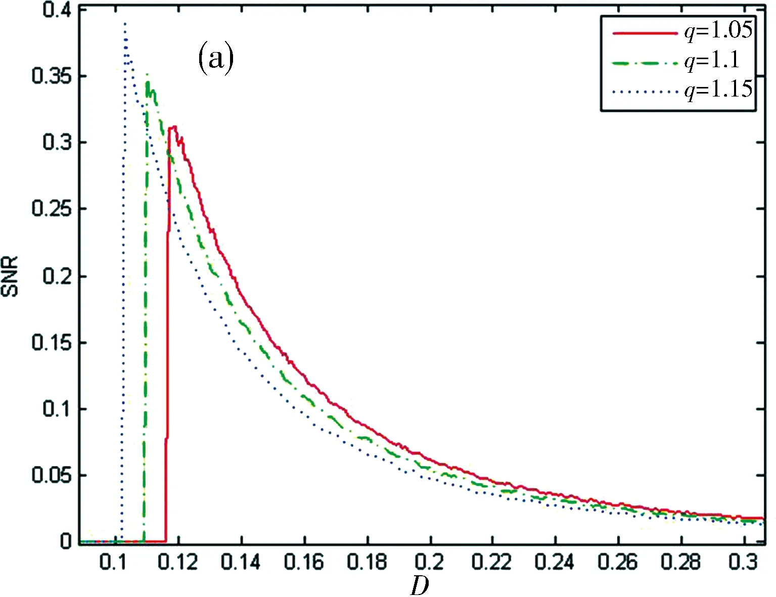
Fig.2 The theoretical results of SNR are plotted as a function of the noise intensity when q varies: (a) characteristics of SNR versus D at Q=3.3; (b) characteristics of SNR versus Q at D=3.3

According to the expression of SNR，the influences of different parameters on the SR are discussed in Fig.2～7.

Fig.2 shows a curve of the SNR as a function of the non-Gaussian noise intensityDand Gaussian noise intensityQ，respectively，for different parameters of the non-Gaussian noise deviation parameterq. In Fig.2(a)，the SNR curve also produces a one-peak structure when noise intensityDis increased，which indicates that stochastic resonance phenomenon appears. The height of the peak is increased and the location of the peak is shifted to small value ofDas deviation parameterqis increased. In Fig.2(b)，with the increase ofQ，there are two peaks in the curves，and the right peak is always larger than the left peak. Firstly，from the figure，it is seen that there appears a weak peak in the SNR curve asQis increased. Then the SNR curve is decreased，which is suppressed to a degree. AsQis continue increased，there appears a pretty peak. It indicates that stochastic resonance phenomenon appears again. The height of the left peak is decreased while the right peak is increased，and the locations of both peaks are shifted to large value ofQas deviation parameterqis increased. It shows that as we choose variable values ofq，the optimal value of noise intensity required is different when stochastic resonance phenomenon appears.

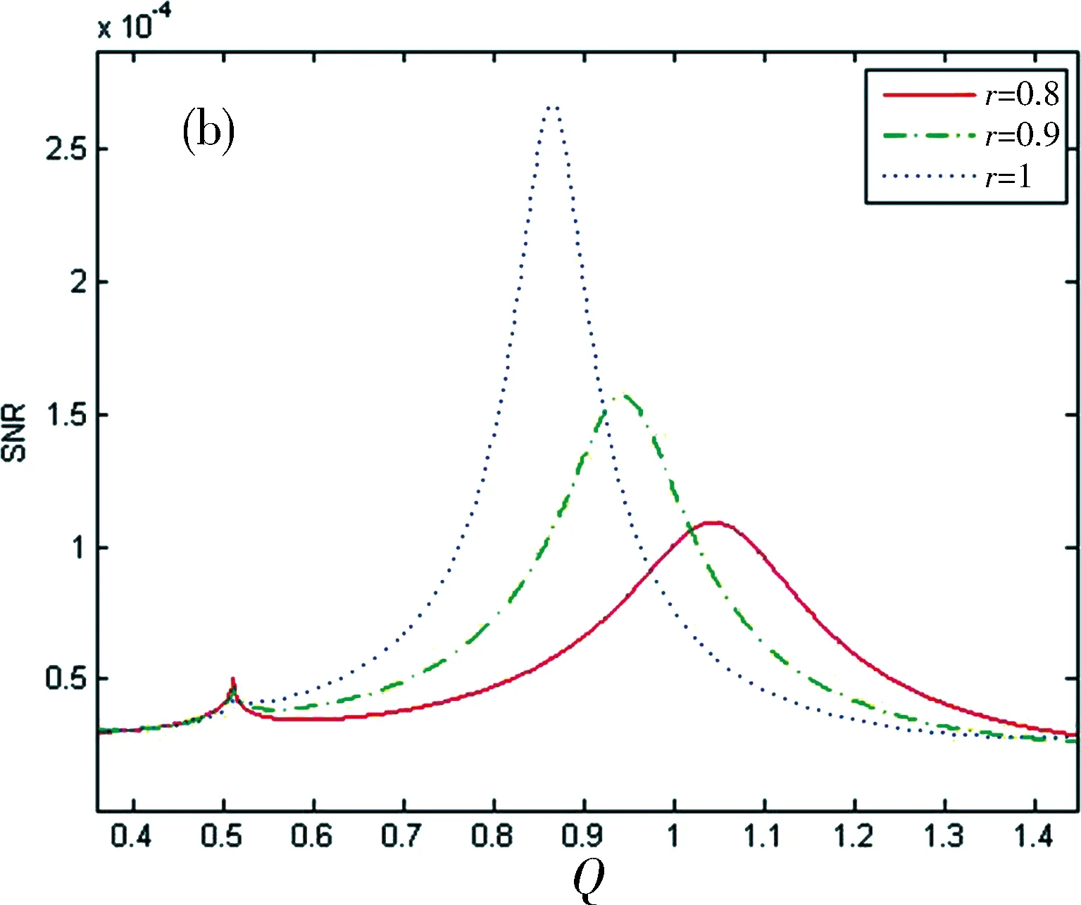
Fig.3 The theoretical results of SNR are plotted as a function of the noise intensity whenτvaries: (a) characteristics of SNR versusD at Q=3.3; (b) characteristics of SNR versus Q at D=3.3

Fig.3 shows a curve of the SNR as a function of the non-Gaussian noise intensityDand the Gaussian noise intensityQ，respectively，for different correlation times of the non-Gaussian noiseτ. In Fig. 3(a)，the SNR curve produces a one-peak structure when noise intensityDis increased，which indicates that conventional stochastic resonance phenomenon appears. The peaks of curves increase as the correlation times of the non-Gaussian noiseτincreases. However，the position of the peak does not shift significantly for differentτ. In Fig. 3(b)，with the increase ofQ，there are two peaks in the curves，and the right peak is always larger than the left peak. The height of the left peak is decreased while the right peak is increased，and the location of both peaks are shifted to small value ofQas correlation times of the non-Gaussian noiseτis increased. It shows that as we choose variable values ofτ，the optimal value of noise intensity required is different when stochastic resonance phenomenon appears.

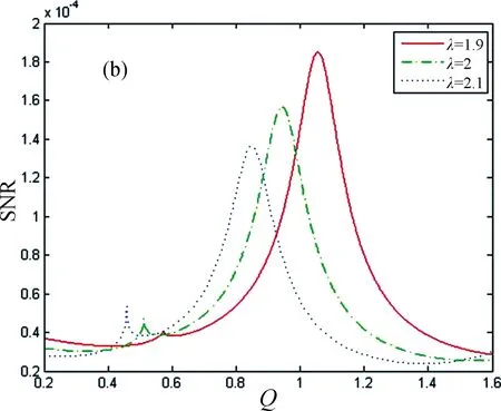
Fig.4 The theoretical results of SNR are plotted as a function of the noise intensity when λ varies: (a) characteristics of SNR versus D at Q=3.3; (b) characteristics of SNR versus Q at D=3.3

Fig.4 shows a curve of the SNR as a function of the non-Gaussian noise intensityDand the Gaussian noise intensityQ，respectively，for different cross-correlation strengthλ. In Fig. 4(a)，the SNR curve produces a one-peak structure when noise intensityDis increased. This is stochastic resonance. The peaks of curves increase as the cross-correlation strengthλincreases. However，the location of the peak is shifted to small value ofDas parameterλis increased. In Fig. 4(b)，there are two peaks in the curves with the increase ofQ. The right peak is always larger than the left peak. The height of the left peak is increased while the right peak is decreased，and the locations of both peaks are shifted to small value ofQas cross-correlation strengthλis increased. It shows that as we choose variable values ofλ，the optimal value of noise intensity required is different when stochastic resonance phenomenon appears. And we can find that there are different influences between Gaussian and non-Gaussian noise under cross-correlation strengthλ.

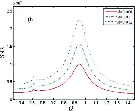
Fig.5 The theoretical results of SNR are plotted as a function of the noise intensity when A varies: (a) characteristics of SNR versus D at Q=3.3; (b) characteristics of SNR versus Q at D=3.3

Fig.5 shows a curve of the SNR as a function of the non-Gaussian noise intensityDand the Gaussian noise intensityQ，respectively，for different amplitudesAof periodic signal. In Fig.5(a)，obviously，the SNR curve produces a one-peak structure when noise intensityDis increased，which indicates that conventional stochastic resonance phenomenon appears. The height of the peak is increased as amplitudesAis increased. And the position of the peak does not shift significantly for differentAwhich is reasonable in physical science. In Fig.5(b)，there are also two peaks in the curves with the increase ofQand the peaks of curves increase asAincreases. Same as before，the position of the peak does not shift significantly for differentA. It shows the system SNR is increased as amplitudesAis increased.

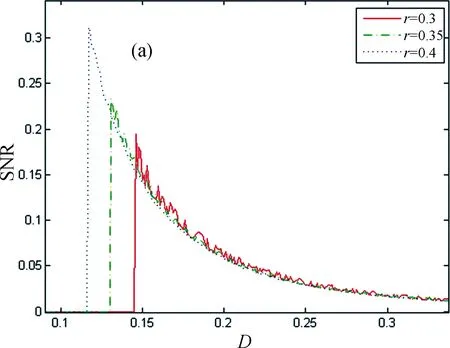
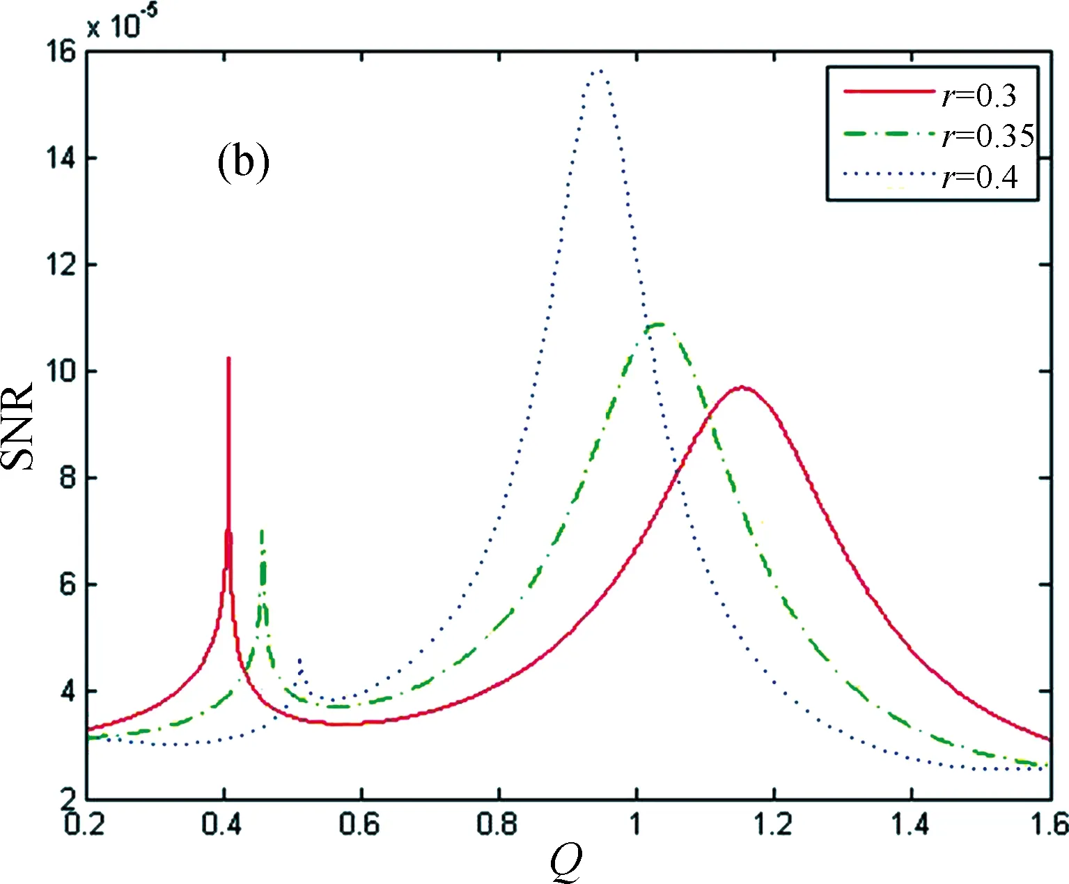
Fig.6 The theoretical results of SNR are plotted as a function of the noise intensity whenrvaries: (a) characteristics of SNR versus D at Q=3.3; (b) characteristics of SNR versus Q at D=3.3

Fig.6 shows a curve of the SNR as a function of the non-Gaussian noise intensityDand the Gaussian noise intensityQ，respectively，for different asymmetric coefficientr. In Fig. 6(a)，the SNR curve also produces an obvious one-peak structure when noise intensityDis increased. This is conventional stochastic resonance. The peaks of curves increase as the asymmetric coefficientrincreases. In Fig.6(b)，with the increase ofQ，there are two peaks in the curves，and the right peak is always larger than the left peak. The height of the left peak is decreased and the location of the left peak is shifted to large value ofQas asymmetric coefficientris increased while the height of the right peak is increased and the location of the right peak is shifted to small value ofQasris increased，which is different from the previous situation.

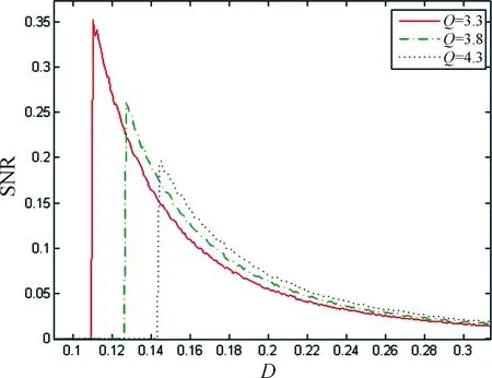
Fig.7 The theoretical results of SNR are plotted as a function of the noise intensity D when Q varies

The SNR as a function of the non-Gaussian noise intensityDfor different Gaussian noise intensitiesQis described in Fig.7. The SNR curve also produces an obvious one-peak structure when noise intensityDis increased. This is conventional stochastic resonance. The peaks of curves decrease as the Gaussian noise intensitiesQincreases. We can see that there is interaction between Gaussian and non-Gaussian noise.

In this paper，we studied the problem of stochastic resonance in an asymmetric nonlinear system driven by periodic signal and correlated noises for a multiplicative non-Gaussian noise and an additive Gaussian white noise in the case. The influence of different parameters on SNR is discussed，including non-Gaussian noise deviation parameter，correlation times of the non-Gaussian noise，cross-correlation strengths，amplitudes of periodic signal，asymmetric coefficient，and both Gaussian and non-Gaussian noise intensities.

From the simulation result，there is a different result when the SNR is a function of the non-Gaussian noise intensity. Firstly，there appears a single peak in the SNR curves as a function of the non-Gaussian noise intensity while there are two peaks in the SNR curves with the increase ofQ. Besides，as different parameters change，there are variation tendency of SNR. Especially，non-Gaussian noise deviation parameterqhas different effect of the non-Gaussian noise on the location of the SNR peak from that of the Gaussian noise，and the cross-correlation strenthλhas different effect of the non-Gaussian noise on the height of the SNR peak from that of the Gaussian noise.