A non-myopic scheduling method of radar sensors for maneuvering target tracking and radiation control

Gan-lin Shan,Gong-guo Xu,Cheng-lin Qiao

Department of Electronic and Optical Engineering,Army Engineering University,Shijiazhuang 050003,China

Keywords:Non-myopic scheduling Radiation control PCRLB POMDP Branch and bound

ABSTRACT In decades,the battle field environment is becoming more and more complex with plenty of electronic equipments.Thus,in order to improve the survivability of radar sensors and satisfy the requirement of maneuvering target tracking with a low probability of intercept,a non-myopic scheduling is proposed to minimize the radiation cost with tracking accuracy constraint.At first,the scheduling problem is formulated as a partially observable Markov decision process(POMDP).Then the tracking accuracy and radiation cost over the future finite time horizon are predicted by the posterior carm'er-rao lower bound(PCRLB)and the hidden Markov model filter,respectively.Finally,the proposed scheduling is implemented efficiently by utilizing the branch and bound(B&B)pruning algorithm.Simulation results show that the performance of maneuvering target tracking was improved by the improved interacting multiple model(IMM),and the scheduler time and maximum memory consumption were significant reduced by the present B&B pruning algorithm without losing the optimal solution.©2020 China Ordnance Society.Production and hosting by Elsevier B.V.on behalf of KeAi Communications Co.This is an open access article under the CCBY-NC-ND license(http://creativecommons.org/licenses/by-nc-nd/4.0/).

1.Introduction

One of the most successful techniques to improve the performance of target tracking system is sensor scheduling[1-3].Sensor scheduling is myopic if it only performs one step ahead in the future.Although the myopic scheduling has low computational and memory cost,sometimes the performance of myopic sensor scheduling is poor.By contrast,the non-myopic scheduling which performs multi-step ahead in the future is better[4,5].A typical objective of sensor scheduling is to select sensor to minimize the tracking cost under constraints over time.In Refs.[6-8],the objective is to minimize the tracking error with dwell time constraint[6],dwell time constraint[7],power constraint[8,9]and sensor resource constraints[10],respectively.In fact,on the other hand,the tracking error is often considered as a constrain[11,12].For example,the objective is to minimize the energy consumption subject to tracking accuracy constrain in the wireless sensor network[12].

In this paper,we consider a sensor scheduling scenario where multiple active sensors track a maneuvering target in the combat system.As the emitting energy can be captured by enemy surveillance sensors,the radiation cost of the combat system is more important than the other factors such as energy consumption[13].In the active/passive multi-sensor system,the radiation cost is calculated by the times of active sensor selection as the passive sensor cannot emit energy[14].In order to further control the radiation,the radiation cost is quantized in Ref.[15],different active sensors are set as different fixed cost,then a simulation-based Q value approximation method is utilized to obtain suboptimal solution.How ever,this approach is usually not suitable for the practice situation.Moreover,using the interception probability factor to measure the radiation cost is another common method[16-19].For example,combining with low probability of intercept(LPI),the entropy of all the sensors with no interception is denoted as the radiation cost in Ref.[16].But,as the prior know ledge of the enemy parametric windows is difficult to obtain,it is hard to compute the interception probability.To avoid this problem,the emission level impact(ELI)is used to represent the radiation cost instead of the interception probability in Refs.[20,21].How ever,the goal of the above work is to trade off the radiation cost and tracking performance that is traditionally been ill-suited for achieving specific control objectives in the combat system[22],and the balance coefficient is always given based on empirical value[15].In addition,the target is almost assumed as non-maneuvering target in the above work.In fact,to dodge tracking,the target is always maneuvering.The interacting multiple model(IMM)algorithm is simple and practical method for maneuvering target tracking.It has been applied to many sensor scheduling systems to track maneuvering target[23-25].As we know,the crucial feature of sensor scheduling is predictable,then how to obtain the predicted tracking accuracy is important.In Ref.[23],the predicted tracking accuracy is obtained without utilizing the measurement,and an adaptive resource management algorithm is proposed to reduce the LPI in radar network.Obviously,the predicted tracking error is larger than the estimated tracking error,sometimes the resource management scheme may not be an optimal scheme.To solve this issue,the predicted tracking accuracy is calculated with a model index prediction algorithm in Refs.[24,25].How ever,the studies of[23-25]are all myopic scheduling,and few researches of non-myopic scheduling for maneuvering target tracking and radiation control are exist.

In this work,it aims to minimize the radiation cost with the tracking accuracy constraint which depends on the tactical requirement in the maneuvering target tracking.Firstly,the IMM is improved by using an adaptive Markov transition probability matrix which is modified by the error compression ratio and model probability variance ratio.Then the posterior carm'er-rao lower bound(PCRLB)is utilized to predict the tracking accuracy.Secondly,the radiation cost is represented by ELI and it is predicted by using hidden Markov model(HMM)filter.Finally,the branch and bound(B&B)pruning algorithm with the suboptimal lower bound is proposed to solve the exponential computational grow th problem.

2.Problem formulation

In this paper,we consider a typical target tracking scenario.There are N active sensors distributed in a sensor field to track a maneuvering target.As the system state is not directly observable,we formulate the scheduling problem as a POMDP.

2.1.Action space and system state

To represent the sensor assignment,the sensor scheduling action at time step k+1 is denoted by,where the vector element=1 or=0 specifies whether the sensor n is active or inactive at time step k+1.For clarity and easy of presentation,all the sensors are independent of each other and only one sensor per time step is activated to track target.

In this paper,the system state vector Skconsists of the target state Xkand the ELI state Ek.Then it can be written as

where［xk，yk，zk］represents the target position and［˙xk，˙yk，˙zk］is the corresponding velocity.Enkdenotes the cumulative received radiation registered by the enemy surveillance system from sensor n（n=1，…，N）till time step k[20].The superscript T represents transpose.

For maneuvering target tracking,the target state Xkcan be estimated efficiently by IMM[25].Therefore,the dynamic state evolves according to the target motion model as

where Fmis the state transition matrix of model m（1，…，M）and M is the number of model.wkdenotes the zero-mean white Gaussian process noise with covariance matrix Q.

According to Ref.[20],the ELI state is quantized to a finite set｛1，…，Ns｝,each value corresponding to a physical threat level and Nsis highest threat level.Then the ELI state can be transited by several transition matrices Tnk（n=1，…，N）.If the sensor n is activated to track target,then

2.2.Observation

Similarly,the system observation vector Zkcan be written as

where ZXkand ZEkare the target measurement and the ELI measurement,respectively.

Moreover,the target measurement ZXkis produced by the sensor measurement model which can be given as

where g denotes the measurement function of the selected sensor and vkis assumed as a zero-mean white Gaussian measurement noise.For the active sensors,the measurement includes range rk,azimuth θkand elevation φk

2.3.Optimization function

We denote a scheduling sequence by a H-tupleak+1，…，ak+H-1］,where H is the prediction time horizon.At any given time k,the goal is to obtain the optimal scheduling sequencein order to minimize the radiation cost while maintaining a desired tracking accuracy.Obviously,there are NHpossible scheduling sequences.Moreover,we define the radiation cost function at time step k+h-1 by r（ak+h-1）which is the sum of all selected sensor ELI states.Then the optimization function is described as

Since the system state is not directly observable,a POMDPkeeps scheduling of the belief state[3].We definewhere bXkand bEkdenote target belief state and ELI belief state,respectively.Then equation(8)can be further stated as

where symbol Erepresents expectation.

3.Problem solution

Fig.1 shows the flow chart of the proposed non-myopic scheduling method.At time step k,the non-myopic scheduling process can be described as follow s:

Step 1:Initialization.Get the target state Xkand the ELI belief state bEkat time step k.

Step 2:Predict the tracking accuracy and the radiation cost in the future,then search the optimal sensor scheduling sequence φk:k+H-1by improved decision tree searching algorithm.

Step 3:Select the first action akin the optimal sensor scheduling sequence φk:k+H-1to control the radar sensor.

Step 4:k=k+1,get the system observation vector Zk+1.If the task is not finished,update the target state and ELI belief state by improved IMM algorithm and HMM,respectively,and then go to Step 1.Otherwise,go to Step 5.

Step 5:End.

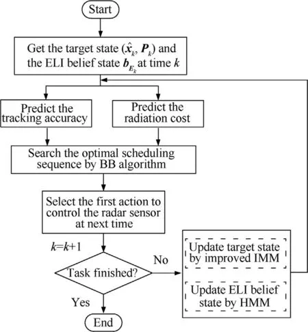
Fig.1.Flowchart of non-myopic scheduling method.

3.1.Adaptive Markov transition probability matrix

As it know n,the IMM is always utilized to track maneuvering target.How ever,the fixed Markov transition probability matrix is always inaccurate and it does not fully describe the conversion between different models during the filtering.In fact,when the target motion state has a tendency to a motion model,the corresponding transition probability should be increased.According to this idea,the posterior information is utilized to revise the Markov transition probability matrix.Here,the posterior information consists of the error compression ratio[26]and the model probability variance ratio.

We define the error compression ratio as

Then the transition probability is modified as

Obviously,the matching model information is magnified and the non-matching models information is omitted in(11).How ever,the modified transition probability matrix may be a non-positive matrix[25].Therefore,two necessary conditions are given as

·As the transition probability matrix is a diagonally-dominant matrix,the second necessary condition is given as

Furthermore,as the error compression ratio only consider the current model information without considering the history model information,sometimes this method is not stable and accurate.To solve this issue,we utilize the model probability variance ratio to further modify the transition probability matrix.

As the transition probability is nonnegative,we define the model probability variance ratio κjkas

It can be seen that when the model probability of model j is increased,κjk＞1.Otherwise,κjk＜1.Based on this,κjkis used to further modify the transition probability matrix.It is described as

Note that the sum of all the elements of each row in the transition probability matrix may not equal to one.Thus the normalization process is stated as

3.2.PCRLB for tracking accuracy prediction

As the further measurements cannot be obtained at the current time step,then the PCRLB is utilized to predict the target tracking accuracy.As it know n,PCRLB is the inverse of the Fisher information matrix(FIM)and expresses the lower bound on the tracking error.Denoting the FIM by Jk,then it is calculated recursively as

with

How ever,the mk+1cannot be obtained at time step k.To obtain the predicted model index,the model probabilityμkyielded by IMM algorithm is used as

where μikrepresents the model probability of motion model i.

Consequently,the procedure of the propose tracking accuracy prediction is described as

Step 1:Obtain the target statecovariance matrix Pkand model probability μkfrom the target belief state bXkwhich is estimated by IMM.

Step 2: Predict the target motion model ~mk+h=

Step 3:Calculate the FIM Jk+hby using Eq.(17).

Step 4:Compute the predicted tracking accuracy

3.3.HMM for radiation cost prediction

Specifically,to use the basic theory of HMM to derive,the system state at current time should be only related to the state at previous time.Due to the continuity of target motion,the target state and radiation state meet the above requirements.Therefore,after the ELI measurement ZEk+1is achieved by the selected sensor n,the ELI belief state can be updated as

where symbol⊗denotes Hadamard product,and“1”is a Ms-dimensional unit column vector.

As ZEk+1cannot be achieved at time step k,its distribution probability is given as

Then the ELI belief state prediction is stated as

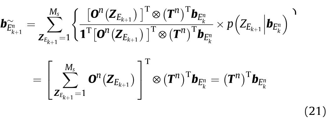
Moreover,the one step radiation cost is calculated as

where Dn=［1，…，Ns］Tis a vector w hose element denotes the nature number in｛1，…，Ns｝.

Therefore,the total radiation cost over the future H time steps is stated as

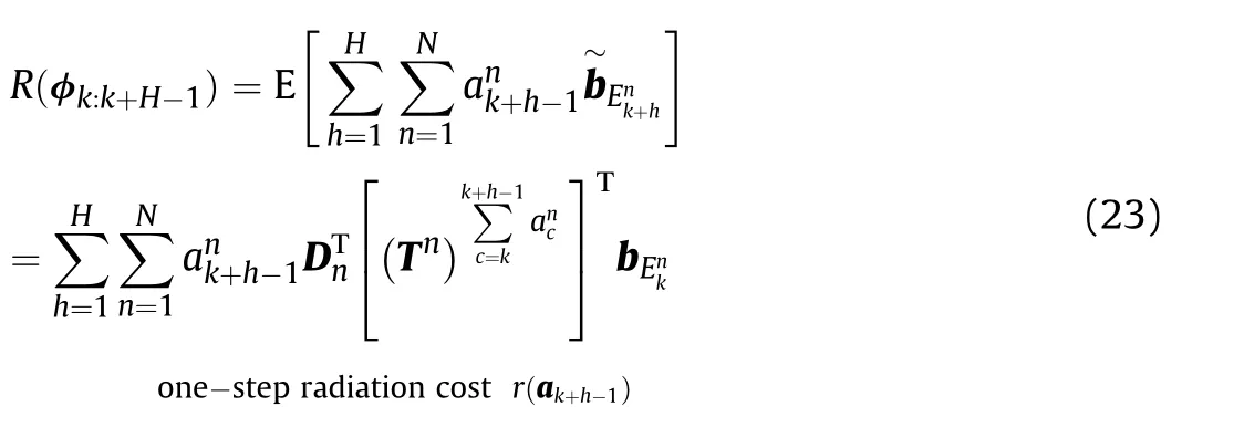
From the derivation process,unlike the commonly used interception probability method,using the HMM to derive the radiation cost is in line with the actual situation.It is not necessary to know the working parameters of enemy targets,which can be well applied to the target tracking process.

3.4.B&B pruning algorithm for sensor scheduling

We translate the sensor scheduling problem in Section 2.3 to a decision tree optimization problem.The depth and branching factor of the tree are equal to the time horizon length and the number of sensors,respectively.Fig.2 shows a decision tree of N=4 and H=3.We de f ine each depth-h（h=1，…，H）node aswhere is the node position.As shown in Fig.2,the decision tree is expanded by the scheduling actions［ak，…，ak+H-1］,and each path from the root to a leaf node corresponds to one possible sensor scheduling sequence.

Therefore,our objective is to find the optimal path with the lowest radiation cost such that the tracking accuracy is maintained within a desired level at each time step.Obviously,searching all the possible paths is computationally infeasible.As a result,it becomes imperative to develop an efficient search technique to reduce the search effort.

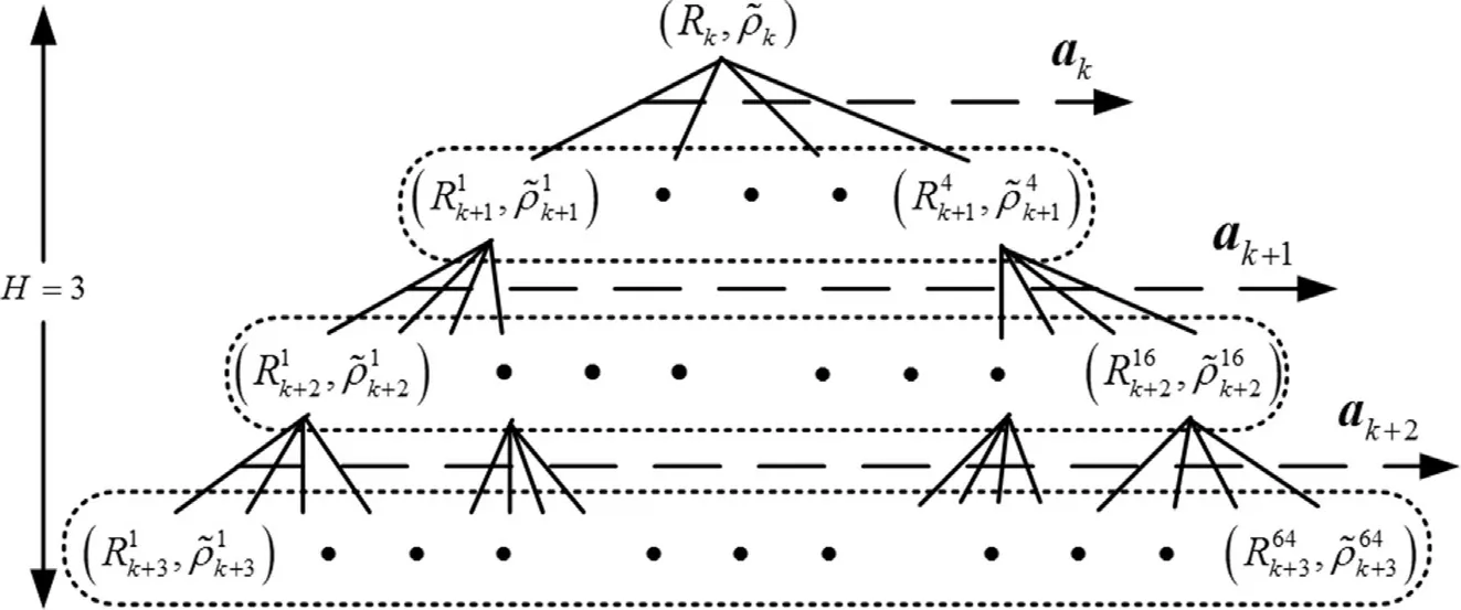
Fig.2.An illustrative decision tree with N=4 and H=3.

The branch and bound pruning algorithm is often utilized to prune redundant branches in the decision tree.How ever,there are two necessary conditions for its application.The first necessary condition is that each node lower bound on the cost is easier to obtain with respect to the actual cost.Another one is the one step cost must be non-negative to ensure the cost of any children of this node is greater than itself.Fortunately,the above conditions are all satisfied in our scheduling problem.By means of the lower bound,the tree is efficiently pruned.Then any node whose lower bound is smaller than the current minimum cost is expanded first.On the other hand,any node which has a bigger lower bound is pruned.

We assume that a node is reached by utilizing the scheduling sequence φk:k+h-1= ［ak，…，ak+h-1］.Then the low er bound L（φk:k+h-1）of this node is stated as

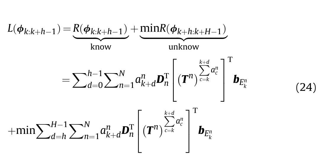
For any given ELI state transition matrix Tn（n=1，…，N）,there is a total of NH-hdistinct values of R（φk+h:k+H-1）.Therefore,it is difficult to obtain the optimal lower bound of R（φk+h:k+H-1）,then a suboptimal lower bound is utilized to instead of it.For each possible sensor sequence φk+h:k+H-1,we have assumed that the tracking accuracy of each possible sensor sequence is maintained with the desired level at each of the future H-h time steps.Then the radiation cost R（φk+h:k+H-1）is translated to a function of Tn.Consequently,the suboptimal low er bound of R（φk+h:k+H-1）is stated as

Moreover,the suboptimal lower bound of L（φk:k+h-1）is written as

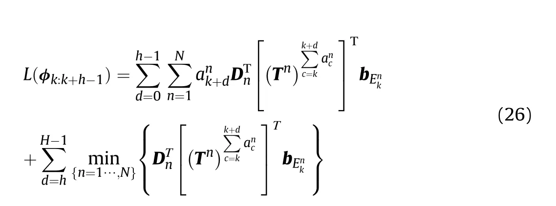
Obviously,there are only a total of N（H-h）nodes should be opened to obtain the suboptimal lower bound,and the calculation of tracking accuracy is not required in this process.As a result,the B&B pruning algorithm for sensor scheduling is shown in Algorithm 1.

Algorithm 1 B&B pruning algorithm.

4.Simulation results

Effectiveness of the proposed sensor scheduling is validated through Monte Carlo simulations.As is shown in Fig.3,in our simulations,four active sensors are utilized to track a maneuvering target.The initial target position and velocity are（15，4，5）km and（-280，-260，0）m/s,respectively.The sampling interval is Ts=1 and the simulation duration is 100s.Without loss of generality,we assume that there are three models are employed:the nearly constant velocity(NCV)model,nearly left constant turn(NLCT)model and nearly right constant turn(NRCT)model.Then the target turns right with ω=-5°during 26 s-50 s,turns left with ω=5°during 51 s-74 s,and maintains uniform motion during the other time.Moreover,the initial model probability is μ=［0.8，0.1，0.1］Tand the initial model switching probability matrix is πij=0.025（i≠j）.

As is shown in Fig.3,sensor 1,sensor 2,sensor 3,and sensor 4 are deployed at（0，-5，0）km,（-5，0，0）km,（5，0，0）km,and（0，5，0）km,respectively.Moreover,the other working parameters of sensors can be summarized as

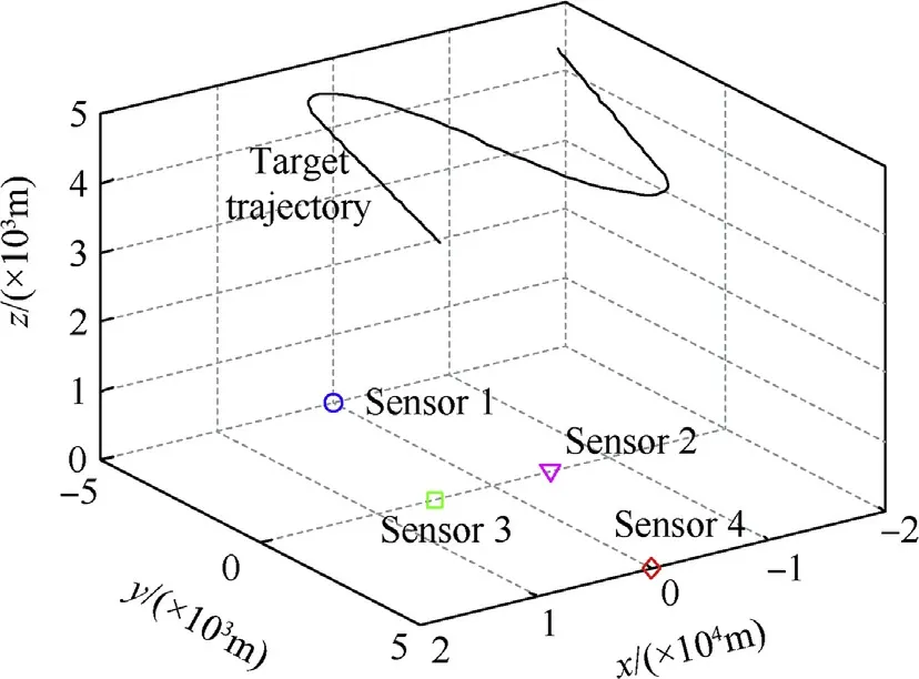
Fig.3.Diagram of the simulation scenario.

sensor 1:σr1=200 m，σθ1=σφ1=0.01 rad

sensor 2:σr1=100 m，σθ1=σφ1=0.005 rad

sensor 3:σr1=100 m，σθ1=σφ1=0.005 rad

sensor 4:σr1=10 m，σθ1=σφ1=0.001 rad

where σrn,σθnand σφnare the standard deviation of range noise,azimuth noise and elevation noise of sensor n（n=1，…，4）,respectively.It can be seen that sensor 1 is more unlikely to increase the ELI but with the worst tracking performance.Sensor 4 has the best tracking performance but it is more likely to increase the ELI.Then we quantize the ELI state as｛1，2，3｝whose element denotes different threat level.Similarly,the ELI measurement is quantized as｛1，2，3｝w hose element denotes different increment in the threat level.Furthermore,the ELI state transition matrices are

Each simulation result is averaged over 200 Monte Carlo simulation runs.

4.1.Comparison of IMM algorithms

To show the advantage of our proposed improved IMM(I-IMM),the standard IMM(SIMM)and IMM with the error compression ratio(EIMM)[23]are used for comparison.The root mean-square error(RMSE)curves of the target position and velocity are shown in Fig.4.Fig.5 shows the model probability of the three algorithms.

It can be seen in Fig.4 that the target position and velocity RMSE curves of I-IMM algorithm are generally lower than EIMM and SIMM algorithms,and the improvement of the target speed is more obvious.It is because that I-IMM algorithm utilizes the error compression ratio and the variance ratio of model probability to modify the probability transition matrix.The matching probability of the model is highest during the target tracking process.Therefore,the corresponding target position and velocity RMSE are smallest.The target position and velocity RMSE curves of EIMM is only better than SIMM when the target moves with NRCT and NLCT.It is because that EIMM algorithm only utilizes the error compression ratio to modify the probability transition matrix,which is not sensitive to the change of target motion mode.Moreover,as the model probability of the three algorithms are inaccurate during the model switching,the tracking error in position and velocity of the three algorithms are comparatively large,which is in line with the actual situation.

Fig.4.Position and velocity RMSE versus time step,(a)position RMSE and(b)velocity RMSE.

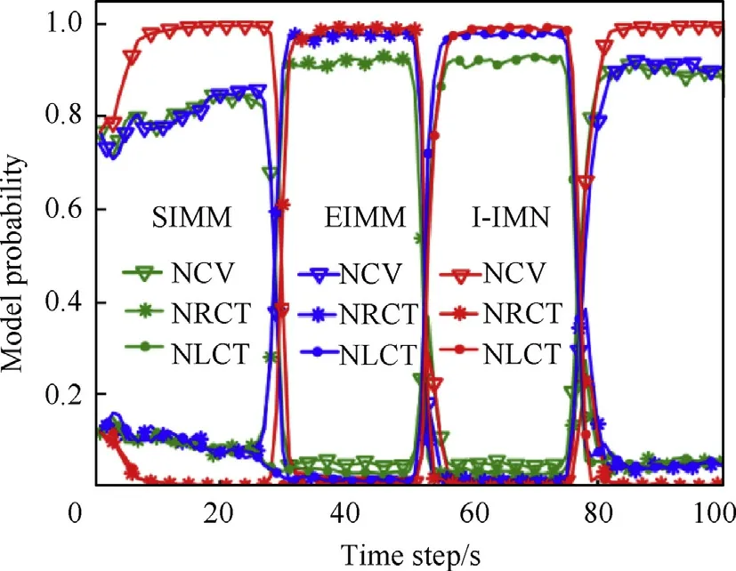
Fig.5.Comparison of the model probability.

Besides,it can be seen in Fig.5 that the model probability of the matching model of I-IMM is generally highest all the time step.Meanwhile,the performance of EIMM performs better than SIMM in model probability when the target moves with NRCT and NLCT.In general,the higher the matching probability is,the higher the tracking accuracy is.It is consistent with the results in Fig.4,which proves the effectiveness of the improved strategy of I-IMM.

4.2.Comparison of pruning algorithms

Next,we compare the pruning performance of enumerative search(ES),uniform cost search(UCS)and B&B.Table 1 summarizes the pruning statistics which include the average number of nodes opened and the maximum number of nodes stored for the case of ρth=50 m.As it know n,the memory consumption and the scheduler time are proportional to the maximum number of nodes stored and average number of nodes opened,respectively[4].It can be seen that both the average number of nodes opened and the maximum number of nodes stored of B&Bare relatively lower than UCS.Moreover,as the decision step H increases,the advantage of B&Bis more obvious.Thus the percentage of the average number of nodes opened decreases faster.Fig.6 shows the percentage of node opened versus time step for the case of decision step H=3.It is evidently that the pruning performance of B&B is better than UCS all the time.

It is obvious in Fig.7 that the cumulative radiation cost is decreasing with H.Then the necessity of the proposed non-myopic scheduling is proved by this result.Considering the computation complexity,we choose H=3 in the next simulations.

4.3.Comparison of scheduling policies

In this simulation,firstly,each sensor is used separately to track the target to show differences in tracking performance of different sensors with different sensor precision.Similar results are shown in Fig.8.It can be seen that the position RMSE of the sensor 1 is the largest and the position RMSE of the sensor 4 is smallest,which correspond to the working parameters of the radar sensors.However,although the tracking error of sensor 4 is small,sensor 4 cannot be used for tracking all the time.Because the radiation cost of sensor 4 will be very large when it is used for tracking all the time.Therefore,it is necessary for the radar sensors to cooperate with each other to reduce the radiation cost and ensure high target tracking accuracy.

Moreover,to investigate the performance of our proposed scheduling(PS),three other scheduling methods are utilized for comparison.There are closest scheduling(CS),myopic scheduling(MS)and myopic scheduling with standard IMM(SMS).

We schedule the sensors for the desired tracking accuracy ρth=20 m,30 m,40 m,50 m,60 m,70 m and 80 m.Figs.9(a)and(b)show the position RMSE curves for the case of ρth=30 m and ρth=50 m.As the CS RMSE does not change for different desired tracking accuracy and in order to show the performance of the other scheduling methods clearly,Fig.9(b)does not show the CS RMSE curve.We note that the position RMSE curves of SMS,MS and PS are generally below the desired tracking accuracy ρthexpect during the model switching.It indicates that the scheduling methods aid in satisfying the desired tracking accuracy.By contrast,the CS RMSE curve does not meet the desired tracking accuracy.Furthermore,as the model probability is inaccurate during the model sw itching,the corresponding RMSE curves are above ρth.Similar results can also obtained for other values of ρth.

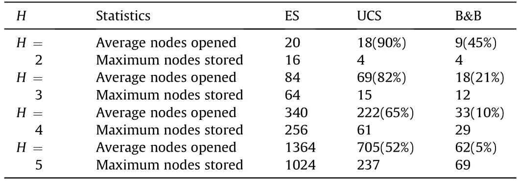
Table 1 Comparisons of pruning algorithms.

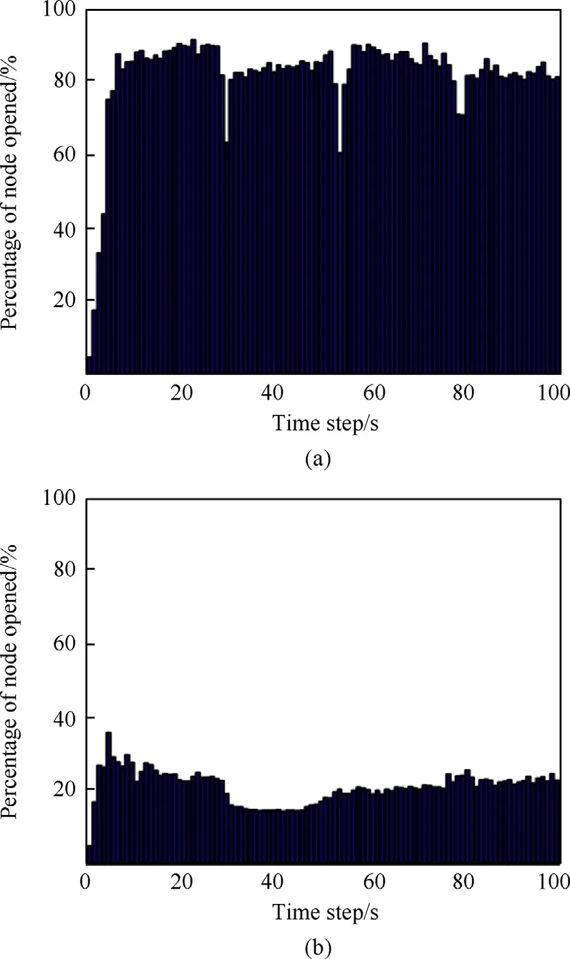
Fig.6.Percentage of node opened versus time step,(a)UCS and(b)B&B.

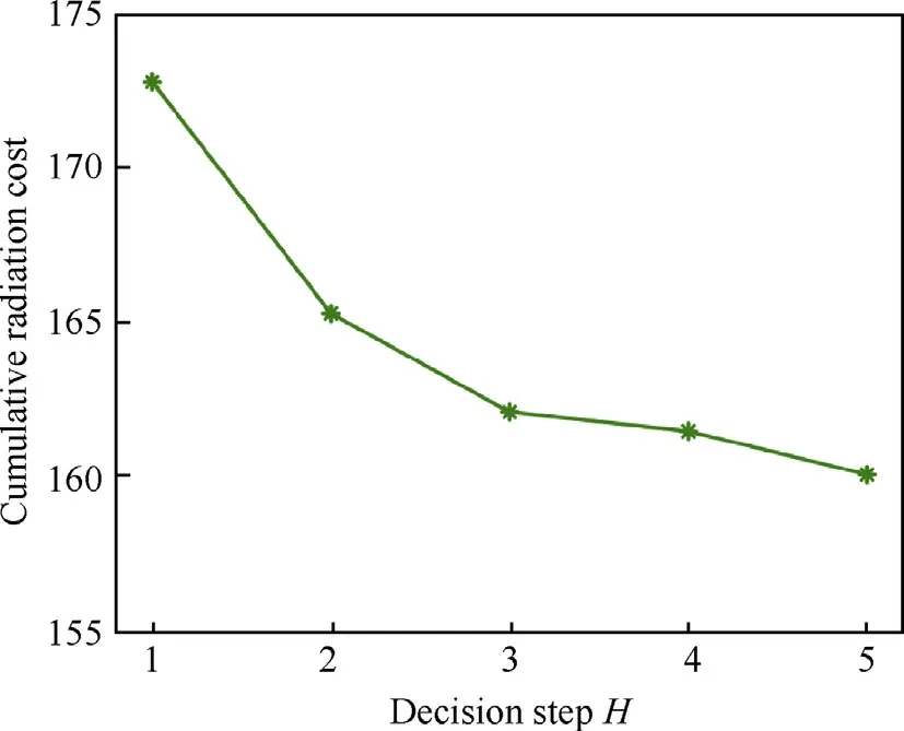
Fig.7.Cumulative radiation cost versus decision step H.

Fig.10 compares the cumulative radiation cost for different desired tracking accuracy.We can clearly find in Fig.10 that the cumulative radiation cost can be reduced efficiently for different desired accuracy by using SMS,MS and PS,respectively.Moreover,as the SMS utilizes the standard IMM for target tracking,the predicted tracking error is always comparatively large.Then it will activate more accurately sensor,such as sensor 4 which is more likely to increase the ELI.Thus the cumulative radiation cost of SMS is larger than MS and PS.Furthermore,it is obvious that the PS can always obtain the minimum cumulative radiation cost,as the PS can find better sensor sequence for target tracking than MS.Fig.11 shows the comparison of cumulative radiation cost and for the case of ρth=50 m.It can be seen that the cumulative ELI value is almost equal to the cumulative radiation cost.Consequently,the effectiveness of the optimization function is proved.

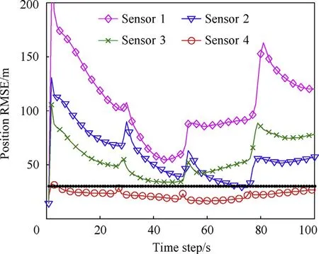
Fig.8.Position RMSE versus different sensors.

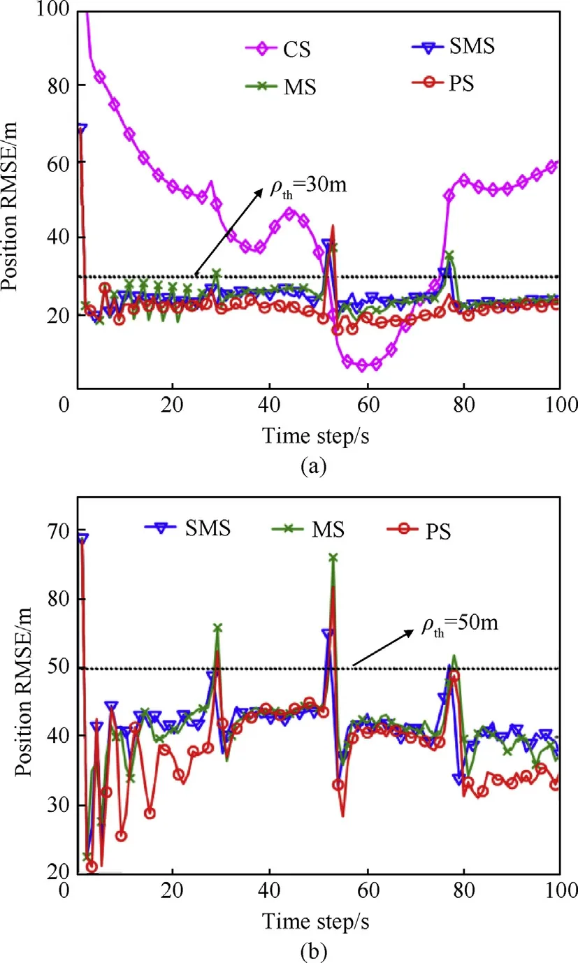
Fig.9.Position RMSE versus time step,(a)ρth=30m and(b)ρth=50m.

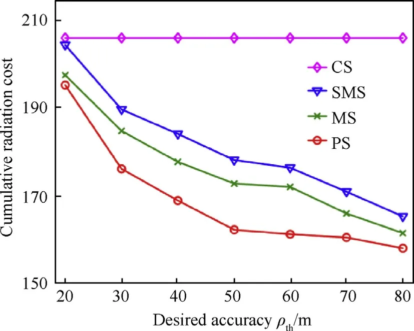
Fig.10.Cumulative radiation cost versus desired tracking accuracy.

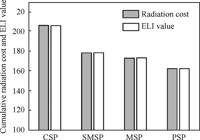
Fig.11.Comparison of cumulative radiation cost and ELI value.

Besides,it can be seen from the experimental results that this paper focuses on the sensor selection strategy to control the radiation cost,which does not discuss the specific working parameters of the sensor.But,the proposed sensor scheduling method is also effective when considering the specific working parameters.We only need to modify the optimization objective or the constraint of the proposed scheduling method.For example,when considering the sensor dwell time,the constraint of sensor switching frequency should be added.When considering the bandwidth and transmit power,the initial level of ELI state should be modified.Specifically,the sensor with large transmit power has a large ELI state.In the future,more detailed researches about the other working parameters will be addressed.

5.Conclusions

The goal in this paper is to control the sensor system radiation cost under the constrain of tracking error by using non-myopic scheduling.We formulated this sensor scheduling problem as a POMDP,and an improved IMM algorithm is presented.To reduce the computation of non-myopic scheduling problem,the B&B pruning algorithm with the suboptimal lower bound was presented.Simulation results indicated that the performance of maneuvering target tracking was improved by the improved IMM,and the scheduler time and maximum memory consumption were significant reduced by the present B&B pruning algorithm without losing the optimal solution.But,the start delay is not considered during sensor scheduling process.Therefore,how to reduce the influence of start delay on sensor scheduling is a future research direction.On the other hand,study on sensor scheduling methods in the clutter environment is another research direction.

Declaration of competing interest

The authors declare that they have no conflicts of interest to this work.We also declare that we do not have any commercial or associative interest that represents a conflict of interest in connection with the work submitted.

Acknowledgement

This work is supported by the National Defense Pre-research Foundation of China(012015012600A2203).